xcube
![]()

New level: Level 9 - spyndex + xcube!
This level shows an example how to calculate all spectral indices provided by Sentinel-2 data using spyndex on the fly. This is done in two steps:
Sentinel-2 data is lazily loaded from Sentinel Hub using xcube and its Sentinel Hub plugin xcube_sh
All sprectral indices are calculated using spyndex. Note that only the spectral indices are considered which can be provided by Sentinel-2 data. The link between Sentinel-2 band names and expressions used by spyndex is encoded in the second part of this notebook.
For this level you need spyndex, xcube, and xcube-sh. To install, run the following commands:
$ conda install -c conda-forge spyndex
$ conda install -c conda-forge xcube
$ conda install -c conda-forge xcube-sh
Note that xcube-sh can be only installed via conda or from source.
Let’s get started: First import everything we need:
[11]:
import spyndex
from xcube.core.store import new_data_store
from xcube.core.maskset import MaskSet
To access Sentinel Hub, you need to create a client ID and client secret on https://identity.dataspace.copernicus.eu/auth/realms/CDSE/account/#/ in the Sentinel Hub dashboard and add them to the credentials dictionary:
[13]:
credentials = {
    "client_id": "xxxxx",
    "client_secret": "xxxxx"
}
Define the selection parameters for the Sentinel Hub data store. The data is taken from Sentinel-2 Level 2a. The area around Lake Constance is selected for the full year of 2020.
[14]:
# data ID of Sentinel-2 Level 2a
data_id = "S2L2A"
# bounding box [west, south, east, north]
bbox = [9, 47, 10, 48]
# bounds of time range
time_range = ("2020-01-01", "2020-12-31")
# spatial resolution in degree equivalent to 20m in latitude direction
spatial_res = 0.00018
# size of chunk
tile_size = [1024, 1024]
Create a Sentinel Hub data store, where the credentials are used during the initialization of the store.
[15]:
store = new_data_store(
    "sentinelhub",
    client_id=credentials["client_id"],
    client_secret=credentials["client_secret"],
    instance_url="https://sh.dataspace.copernicus.eu",
    oauth2_url=(
        "https://identity.dataspace.copernicus.eu/auth/"
        "realms/CDSE/protocol/openid-connect"
    )
)
Open the data with the given selection parameters. The function translate_bands links the Sentinel-2 band names to the band expressions. Furthermore, only the band expressions are considered, which are provided by Sentinel-2.
[16]:
# new functions working with spyndex
def translate_bands():
    bandid_translator = {}
    for band in spyndex.bands:
        if hasattr(spyndex.bands.get(band), "sentinel2a"):
            s2_band = spyndex.bands.get(band).sentinel2a.band
            s2_band = s2_band[0] + s2_band[1:].zfill(2)
            bandid_translator[band] = s2_band
    return bandid_translator


# open dataset
variable_names = list(translate_bands().values())
variable_names.append("SCL")
ds = store.open_data(
    data_id,
    variable_names=variable_names,
    bbox=bbox,
    spatial_res=spatial_res,
    time_range=time_range,
    tile_size=tile_size,
)
ds
/home/konstantin/miniconda3/envs/spyndex/lib/python3.12/site-packages/xcube_sh/sentinelhub.py:254: UserWarning: The argument 'infer_datetime_format' is deprecated and will be removed in a future version. A strict version of it is now the default, see https://pandas.pydata.org/pdeps/0004-consistent-to-datetime-parsing.html. You can safely remove this argument.
  dt = pd.to_datetime(dt, infer_datetime_format=True, utc=True)
/home/konstantin/miniconda3/envs/spyndex/lib/python3.12/site-packages/xcube_sh/sentinelhub.py:317: FutureWarning: 'H' is deprecated and will be removed in a future version. Please use 'h' instead of 'H'.
  pd.to_timedelta(max_timedelta)
[16]:
<xarray.Dataset> Size: 270GB
Dimensions:    (time: 146, lat: 6144, lon: 6144, bnds: 2)
Coordinates:
  * lat        (lat) float64 49kB 48.11 48.11 48.11 48.11 ... 47.0 47.0 47.0
  * lon        (lon) float64 49kB 9.0 9.0 9.0 9.001 ... 10.11 10.11 10.11 10.11
  * time       (time) datetime64[ns] 1kB 2020-01-02T10:27:34 ... 2020-12-30T1...
    time_bnds  (time, bnds) datetime64[ns] 2kB dask.array<chunksize=(146, 2), meta=np.ndarray>
Dimensions without coordinates: bnds
Data variables: (12/13)
    B01        (time, lat, lon) float32 22GB dask.array<chunksize=(1, 1024, 1024), meta=np.ndarray>
    B02        (time, lat, lon) float32 22GB dask.array<chunksize=(1, 1024, 1024), meta=np.ndarray>
    B03        (time, lat, lon) float32 22GB dask.array<chunksize=(1, 1024, 1024), meta=np.ndarray>
    B04        (time, lat, lon) float32 22GB dask.array<chunksize=(1, 1024, 1024), meta=np.ndarray>
    B05        (time, lat, lon) float32 22GB dask.array<chunksize=(1, 1024, 1024), meta=np.ndarray>
    B06        (time, lat, lon) float32 22GB dask.array<chunksize=(1, 1024, 1024), meta=np.ndarray>
    ...         ...
    B08        (time, lat, lon) float32 22GB dask.array<chunksize=(1, 1024, 1024), meta=np.ndarray>
    B09        (time, lat, lon) float32 22GB dask.array<chunksize=(1, 1024, 1024), meta=np.ndarray>
    B11        (time, lat, lon) float32 22GB dask.array<chunksize=(1, 1024, 1024), meta=np.ndarray>
    B12        (time, lat, lon) float32 22GB dask.array<chunksize=(1, 1024, 1024), meta=np.ndarray>
    B8A        (time, lat, lon) float32 22GB dask.array<chunksize=(1, 1024, 1024), meta=np.ndarray>
    SCL        (time, lat, lon) uint8 6GB dask.array<chunksize=(1, 1024, 1024), meta=np.ndarray>
Attributes:
    Conventions:             CF-1.7
    title:                   S2L2A Data Cube Subset
    history:                 [{'program': 'xcube_sh.chunkstore.SentinelHubChu...
    date_created:            2024-05-17T14:55:01.397072
    time_coverage_start:     2020-01-02T10:27:25.374000+00:00
    time_coverage_end:       2020-12-30T10:37:45.795000+00:00
    time_coverage_duration:  P363DT0H10M20.421S
    geospatial_lon_min:      9
    geospatial_lat_min:      47
    geospatial_lon_max:      10.10592
    geospatial_lat_max:      48.10592
processing_level: L2A- time: 146
- lat: 6144
- lon: 6144
- bnds: 2
- lat(lat)float6448.11 48.11 48.11 ... 47.0 47.0
- units :
- decimal_degrees
- long_name :
- latitude
- standard_name :
- latitude
array([48.10583, 48.10565, 48.10547, ..., 47.00045, 47.00027, 47.00009])
- lon(lon)float649.0 9.0 9.0 ... 10.11 10.11 10.11
- units :
- decimal_degrees
- long_name :
- longitude
- standard_name :
- longitude
array([ 9.00009, 9.00027, 9.00045, ..., 10.10547, 10.10565, 10.10583])
- time(time)datetime64[ns]2020-01-02T10:27:34 ... 2020-12-...
- standard_name :
- time
- bounds :
- time_bnds
array(['2020-01-02T10:27:34.000000000', '2020-01-05T10:37:30.000000000', '2020-01-07T10:27:34.000000000', '2020-01-10T10:37:31.000000000', '2020-01-12T10:27:34.000000000', '2020-01-15T10:37:30.000000000', '2020-01-17T10:27:33.000000000', '2020-01-20T10:37:30.000000000', '2020-01-22T10:27:33.000000000', '2020-01-25T10:37:29.000000000', '2020-01-27T10:27:32.000000000', '2020-01-30T10:37:28.000000000', '2020-02-01T10:27:32.000000000', '2020-02-04T10:37:28.000000000', '2020-02-06T10:27:33.000000000', '2020-02-09T10:37:31.000000000', '2020-02-11T10:27:32.000000000', '2020-02-14T10:37:29.000000000', '2020-02-16T10:27:35.000000000', '2020-02-19T10:37:32.000000000', '2020-02-21T10:27:34.000000000', '2020-02-24T10:37:31.000000000', '2020-02-26T10:27:37.000000000', '2020-02-29T10:37:33.000000000', '2020-03-02T10:27:35.000000000', '2020-03-05T10:37:32.000000000', '2020-03-07T10:27:37.000000000', '2020-03-10T10:37:34.000000000', '2020-03-12T10:27:36.000000000', '2020-03-15T10:37:32.000000000', '2020-03-17T10:27:37.000000000', '2020-03-20T10:37:34.000000000', '2020-03-22T10:27:36.000000000', '2020-03-25T10:37:32.000000000', '2020-03-27T10:27:37.000000000', '2020-03-30T10:37:34.000000000', '2020-04-01T10:27:35.000000000', '2020-04-04T10:37:32.000000000', '2020-04-06T10:27:35.000000000', '2020-04-09T10:37:33.000000000', '2020-04-11T10:27:38.000000000', '2020-04-14T10:37:35.000000000', '2020-04-16T10:27:35.000000000', '2020-04-19T10:37:31.000000000', '2020-04-21T10:27:41.000000000', '2020-04-24T10:37:38.000000000', '2020-04-26T10:27:34.000000000', '2020-04-29T10:37:32.000000000', '2020-05-01T10:27:43.000000000', '2020-05-04T10:37:40.000000000', '2020-05-06T10:27:37.000000000', '2020-05-09T10:37:34.000000000', '2020-05-11T10:27:44.000000000', '2020-05-14T10:37:43.000000000', '2020-05-16T10:27:39.000000000', '2020-05-19T10:37:36.000000000', '2020-05-21T10:27:45.000000000', '2020-05-24T10:37:42.000000000', '2020-05-26T10:27:40.000000000', '2020-05-29T10:37:37.000000000', '2020-05-31T10:27:46.000000000', '2020-06-03T10:37:42.000000000', '2020-06-05T10:27:41.000000000', '2020-06-08T10:37:38.000000000', '2020-06-10T10:27:46.000000000', '2020-06-13T10:37:42.000000000', '2020-06-15T10:27:42.000000000', '2020-06-18T10:37:39.000000000', '2020-06-20T10:27:45.000000000', '2020-06-23T10:37:42.000000000', '2020-06-25T10:27:42.000000000', '2020-06-28T10:37:38.000000000', '2020-06-30T10:27:45.000000000', '2020-07-03T10:37:41.000000000', '2020-07-05T10:27:42.000000000', '2020-07-08T10:37:38.000000000', '2020-07-10T10:27:44.000000000', '2020-07-13T10:37:40.000000000', '2020-07-15T10:27:41.000000000', '2020-07-18T10:37:37.000000000', '2020-07-20T10:27:45.000000000', '2020-07-23T10:37:41.000000000', '2020-07-25T10:27:42.000000000', '2020-07-28T10:37:39.000000000', '2020-07-30T10:27:45.000000000', '2020-08-02T10:37:42.000000000', '2020-08-04T10:27:43.000000000', '2020-08-07T10:37:39.000000000', '2020-08-09T10:27:45.000000000', '2020-08-12T10:37:42.000000000', '2020-08-14T10:27:43.000000000', '2020-08-17T10:37:40.000000000', '2020-08-19T10:27:45.000000000', '2020-08-22T10:37:42.000000000', '2020-08-24T10:27:43.000000000', '2020-08-27T10:37:39.000000000', '2020-08-29T10:27:45.000000000', '2020-09-01T10:37:41.000000000', '2020-09-03T10:27:42.000000000', '2020-09-06T10:37:39.000000000', '2020-09-08T10:27:43.000000000', '2020-09-11T10:37:40.000000000', '2020-09-13T10:27:42.000000000', '2020-09-16T10:37:38.000000000', '2020-09-18T10:27:44.000000000', '2020-09-21T10:37:41.000000000', '2020-09-23T10:27:42.000000000', '2020-09-26T10:37:39.000000000', '2020-09-28T10:27:45.000000000', '2020-10-01T10:37:42.000000000', '2020-10-03T10:27:43.000000000', '2020-10-06T10:37:40.000000000', '2020-10-08T10:27:45.000000000', '2020-10-11T10:37:42.000000000', '2020-10-13T10:27:43.000000000', '2020-10-16T10:37:40.000000000', '2020-10-18T10:27:47.000000000', '2020-10-21T10:37:41.000000000', '2020-10-23T10:27:43.000000000', '2020-10-26T10:37:39.000000000', '2020-10-28T10:27:46.000000000', '2020-10-31T10:37:41.000000000', '2020-11-02T10:27:42.000000000', '2020-11-05T10:37:38.000000000', '2020-11-07T10:27:44.000000000', '2020-11-10T10:37:40.000000000', '2020-11-12T10:27:40.000000000', '2020-11-15T10:37:37.000000000', '2020-11-17T10:27:44.000000000', '2020-11-20T10:37:38.000000000', '2020-11-22T10:27:40.000000000', '2020-11-25T10:37:36.000000000', '2020-11-27T10:27:42.000000000', '2020-11-30T10:37:36.000000000', '2020-12-02T10:27:39.000000000', '2020-12-05T10:37:35.000000000', '2020-12-07T10:27:37.000000000', '2020-12-10T10:37:32.000000000', '2020-12-12T10:27:36.000000000', '2020-12-15T10:37:32.000000000', '2020-12-17T10:27:39.000000000', '2020-12-20T10:37:34.000000000', '2020-12-22T10:27:36.000000000', '2020-12-25T10:37:33.000000000', '2020-12-27T10:27:41.000000000', '2020-12-30T10:37:36.000000000'], dtype='datetime64[ns]') - time_bnds(time, bnds)datetime64[ns]dask.array<chunksize=(146, 2), meta=np.ndarray>
- standard_name :
- time
Array Chunk Bytes 2.28 kiB 2.28 kiB Shape (146, 2) (146, 2) Dask graph 1 chunks in 2 graph layers Data type datetime64[ns] numpy.ndarray
- B01(time, lat, lon)float32dask.array<chunksize=(1, 1024, 1024), meta=np.ndarray>
- sample_type :
- FLOAT32
- units :
- reflectance
- wavelength :
- 442.45
- wavelength_a :
- 442.7
- wavelength_b :
- 442.2
- bandwidth :
- 21.0
- bandwidth_a :
- 21
- bandwidth_b :
- 21
- resolution :
- 60
Array Chunk Bytes 20.53 GiB 4.00 MiB Shape (146, 6144, 6144) (1, 1024, 1024) Dask graph 5256 chunks in 2 graph layers Data type float32 numpy.ndarray - B02(time, lat, lon)float32dask.array<chunksize=(1, 1024, 1024), meta=np.ndarray>
- sample_type :
- FLOAT32
- units :
- reflectance
- wavelength :
- 492.25
- wavelength_a :
- 492.4
- wavelength_b :
- 492.1
- bandwidth :
- 66.0
- bandwidth_a :
- 66
- bandwidth_b :
- 66
- resolution :
- 10
Array Chunk Bytes 20.53 GiB 4.00 MiB Shape (146, 6144, 6144) (1, 1024, 1024) Dask graph 5256 chunks in 2 graph layers Data type float32 numpy.ndarray - B03(time, lat, lon)float32dask.array<chunksize=(1, 1024, 1024), meta=np.ndarray>
- sample_type :
- FLOAT32
- units :
- reflectance
- wavelength :
- 559.4
- wavelength_a :
- 559.8
- wavelength_b :
- 559
- bandwidth :
- 36.0
- bandwidth_a :
- 36
- bandwidth_b :
- 36
- resolution :
- 10
Array Chunk Bytes 20.53 GiB 4.00 MiB Shape (146, 6144, 6144) (1, 1024, 1024) Dask graph 5256 chunks in 2 graph layers Data type float32 numpy.ndarray - B04(time, lat, lon)float32dask.array<chunksize=(1, 1024, 1024), meta=np.ndarray>
- sample_type :
- FLOAT32
- units :
- reflectance
- wavelength :
- 664.75
- wavelength_a :
- 664.6
- wavelength_b :
- 664.9
- bandwidth :
- 31.0
- bandwidth_a :
- 31
- bandwidth_b :
- 31
- resolution :
- 10
Array Chunk Bytes 20.53 GiB 4.00 MiB Shape (146, 6144, 6144) (1, 1024, 1024) Dask graph 5256 chunks in 2 graph layers Data type float32 numpy.ndarray - B05(time, lat, lon)float32dask.array<chunksize=(1, 1024, 1024), meta=np.ndarray>
- sample_type :
- FLOAT32
- units :
- reflectance
- wavelength :
- 703.95
- wavelength_a :
- 704.1
- wavelength_b :
- 703.8
- bandwidth :
- 15.5
- bandwidth_a :
- 15
- bandwidth_b :
- 16
- resolution :
- 20
Array Chunk Bytes 20.53 GiB 4.00 MiB Shape (146, 6144, 6144) (1, 1024, 1024) Dask graph 5256 chunks in 2 graph layers Data type float32 numpy.ndarray - B06(time, lat, lon)float32dask.array<chunksize=(1, 1024, 1024), meta=np.ndarray>
- sample_type :
- FLOAT32
- units :
- reflectance
- wavelength :
- 739.8
- wavelength_a :
- 740.5
- wavelength_b :
- 739.1
- bandwidth :
- 15.0
- bandwidth_a :
- 15
- bandwidth_b :
- 15
- resolution :
- 20
Array Chunk Bytes 20.53 GiB 4.00 MiB Shape (146, 6144, 6144) (1, 1024, 1024) Dask graph 5256 chunks in 2 graph layers Data type float32 numpy.ndarray - B07(time, lat, lon)float32dask.array<chunksize=(1, 1024, 1024), meta=np.ndarray>
- sample_type :
- FLOAT32
- units :
- reflectance
- wavelength :
- 781.25
- wavelength_a :
- 782.8
- wavelength_b :
- 779.7
- bandwidth :
- 20.0
- bandwidth_a :
- 20
- bandwidth_b :
- 20
- resolution :
- 20
Array Chunk Bytes 20.53 GiB 4.00 MiB Shape (146, 6144, 6144) (1, 1024, 1024) Dask graph 5256 chunks in 2 graph layers Data type float32 numpy.ndarray - B08(time, lat, lon)float32dask.array<chunksize=(1, 1024, 1024), meta=np.ndarray>
- sample_type :
- FLOAT32
- units :
- reflectance
- wavelength :
- 832.85
- wavelength_a :
- 832.8
- wavelength_b :
- 832.9
- bandwidth :
- 106.0
- bandwidth_a :
- 106
- bandwidth_b :
- 106
- resolution :
- 10
Array Chunk Bytes 20.53 GiB 4.00 MiB Shape (146, 6144, 6144) (1, 1024, 1024) Dask graph 5256 chunks in 2 graph layers Data type float32 numpy.ndarray - B09(time, lat, lon)float32dask.array<chunksize=(1, 1024, 1024), meta=np.ndarray>
- sample_type :
- FLOAT32
- units :
- reflectance
- wavelength :
- 944.15
- wavelength_a :
- 945.1
- wavelength_b :
- 943.2
- bandwidth :
- 20.5
- bandwidth_a :
- 20
- bandwidth_b :
- 21
- resolution :
- 60
Array Chunk Bytes 20.53 GiB 4.00 MiB Shape (146, 6144, 6144) (1, 1024, 1024) Dask graph 5256 chunks in 2 graph layers Data type float32 numpy.ndarray - B11(time, lat, lon)float32dask.array<chunksize=(1, 1024, 1024), meta=np.ndarray>
- sample_type :
- FLOAT32
- units :
- reflectance
- wavelength :
- 1612.05
- wavelength_a :
- 1613.7
- wavelength_b :
- 1610.4
- bandwidth :
- 92.5
- bandwidth_a :
- 91
- bandwidth_b :
- 94
- resolution :
- 20
Array Chunk Bytes 20.53 GiB 4.00 MiB Shape (146, 6144, 6144) (1, 1024, 1024) Dask graph 5256 chunks in 2 graph layers Data type float32 numpy.ndarray - B12(time, lat, lon)float32dask.array<chunksize=(1, 1024, 1024), meta=np.ndarray>
- sample_type :
- FLOAT32
- units :
- reflectance
- wavelength :
- 2194.05
- wavelength_a :
- 2202.4
- wavelength_b :
- 2185.7
- bandwidth :
- 180.0
- bandwidth_a :
- 175
- bandwidth_b :
- 185
- resolution :
- 20
Array Chunk Bytes 20.53 GiB 4.00 MiB Shape (146, 6144, 6144) (1, 1024, 1024) Dask graph 5256 chunks in 2 graph layers Data type float32 numpy.ndarray - B8A(time, lat, lon)float32dask.array<chunksize=(1, 1024, 1024), meta=np.ndarray>
- sample_type :
- FLOAT32
- units :
- reflectance
- wavelength :
- 864.35
- wavelength_a :
- 864.7
- wavelength_b :
- 864
- bandwidth :
- 21.5
- bandwidth_a :
- 21
- bandwidth_b :
- 22
- resolution :
- 20
Array Chunk Bytes 20.53 GiB 4.00 MiB Shape (146, 6144, 6144) (1, 1024, 1024) Dask graph 5256 chunks in 2 graph layers Data type float32 numpy.ndarray - SCL(time, lat, lon)uint8dask.array<chunksize=(1, 1024, 1024), meta=np.ndarray>
- sample_type :
- UINT8
- flag_values :
- 0,1,2,3,4,5,6,7,8,9,10,11
- flag_meanings :
- no_data saturated_or_defective dark_area_pixels cloud_shadows vegetation bare_soils water clouds_low_probability_or_unclassified clouds_medium_probability clouds_high_probability cirrus snow_or_ice
Array Chunk Bytes 5.13 GiB 1.00 MiB Shape (146, 6144, 6144) (1, 1024, 1024) Dask graph 5256 chunks in 2 graph layers Data type uint8 numpy.ndarray
- latPandasIndex
PandasIndex(Index([ 48.10583, 48.10565, 48.10547, 48.10529, 48.105109999999996, 48.104929999999996, 48.104749999999996, 48.104569999999995, 48.104389999999995, 48.104209999999995, ... 47.00171, 47.00153, 47.00135, 47.00117, 47.00099, 47.00081, 47.00063, 47.00045, 47.00027, 47.00009], dtype='float64', name='lat', length=6144)) - lonPandasIndex
PandasIndex(Index([ 9.00009, 9.00027, 9.00045, 9.000630000000001, 9.00081, 9.00099, 9.00117, 9.00135, 9.00153, 9.001710000000001, ... 10.104209999999998, 10.104389999999999, 10.104569999999999, 10.10475, 10.10493, 10.10511, 10.10529, 10.105469999999999, 10.105649999999999, 10.10583], dtype='float64', name='lon', length=6144)) - timePandasIndex
PandasIndex(DatetimeIndex(['2020-01-02 10:27:34', '2020-01-05 10:37:30',
               '2020-01-07 10:27:34', '2020-01-10 10:37:31',
               '2020-01-12 10:27:34', '2020-01-15 10:37:30',
               '2020-01-17 10:27:33', '2020-01-20 10:37:30',
               '2020-01-22 10:27:33', '2020-01-25 10:37:29',
               ...
               '2020-12-07 10:27:37', '2020-12-10 10:37:32',
               '2020-12-12 10:27:36', '2020-12-15 10:37:32',
               '2020-12-17 10:27:39', '2020-12-20 10:37:34',
               '2020-12-22 10:27:36', '2020-12-25 10:37:33',
               '2020-12-27 10:27:41', '2020-12-30 10:37:36'],
              dtype='datetime64[ns]', name='time', length=146, freq=None))
- Conventions :
- CF-1.7
- title :
- S2L2A Data Cube Subset
- history :
- [{'program': 'xcube_sh.chunkstore.SentinelHubChunkStore', 'cube_config': {'dataset_name': 'S2L2A', 'band_names': ['B01', 'B02', 'B03', 'B08', 'B8A', 'B04', 'B05', 'B06', 'B07', 'B11', 'B12', 'B09', 'SCL'], 'band_fill_values': None, 'band_sample_types': None, 'band_units': None, 'tile_size': [1024, 1024], 'bbox': [9, 47, 10.10592, 48.10592], 'spatial_res': 0.00018, 'crs': 'WGS84', 'upsampling': 'NEAREST', 'downsampling': 'NEAREST', 'mosaicking_order': 'mostRecent', 'time_range': ['2020-01-01T00:00:00+00:00', '2020-12-31T00:00:00+00:00'], 'time_period': None, 'time_tolerance': '0 days 00:10:00', 'collection_id': None, 'four_d': False}}]
- date_created :
- 2024-05-17T14:55:01.397072
- time_coverage_start :
- 2020-01-02T10:27:25.374000+00:00
- time_coverage_end :
- 2020-12-30T10:37:45.795000+00:00
- time_coverage_duration :
- P363DT0H10M20.421S
- geospatial_lon_min :
- 9
- geospatial_lat_min :
- 47
- geospatial_lon_max :
- 10.10592
- geospatial_lat_max :
- 48.10592
- processing_level :
- L2A
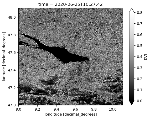
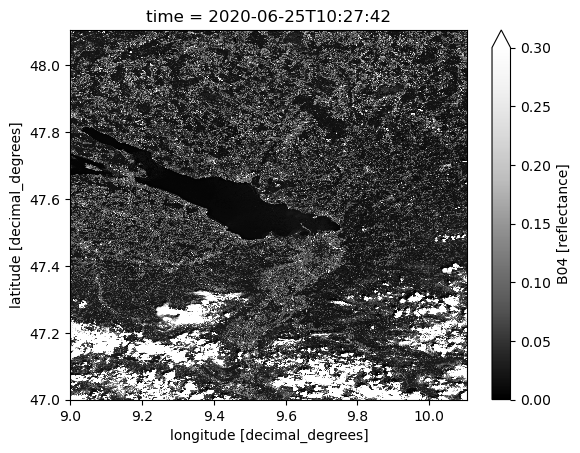
We plot band B04 (red 650nm-680nm) at one time step as an example.
[17]:
ds.B04.isel(time=70).plot.imshow(vmin=0, vmax=0.3, cmap="Greys_r")
[17]:
<matplotlib.image.AxesImage at 0x700a444c43b0>
Here begins the second part namely the calculation of the spectral indices.
Firstly, we filter the dataset where no data is available or where observation is saturated or defective.
[21]:
scene_classif = MaskSet(ds.SCL)
scene_classif
[21]:
| Flag name | Mask | Value |
|---|---|---|
| no_data | None | 0 |
| saturated_or_defective | None | 1 |
| dark_area_pixels | None | 2 |
| cloud_shadows | None | 3 |
| vegetation | None | 4 |
| bare_soils | None | 5 |
| water | None | 6 |
| clouds_low_probability_or_unclassified | None | 7 |
| clouds_medium_probability | None | 8 |
| clouds_high_probability | None | 9 |
| cirrus | None | 10 |
| snow_or_ice | None | 11 |
[22]:
ds = ds.where(~scene_classif.no_data & ~scene_classif.saturated_or_defective)
ds
[22]:
<xarray.Dataset> Size: 287GB
Dimensions:    (time: 146, lat: 6144, lon: 6144, bnds: 2)
Coordinates:
  * lat        (lat) float64 49kB 48.11 48.11 48.11 48.11 ... 47.0 47.0 47.0
  * lon        (lon) float64 49kB 9.0 9.0 9.0 9.001 ... 10.11 10.11 10.11 10.11
  * time       (time) datetime64[ns] 1kB 2020-01-02T10:27:34 ... 2020-12-30T1...
    time_bnds  (time, bnds) datetime64[ns] 2kB dask.array<chunksize=(146, 2), meta=np.ndarray>
Dimensions without coordinates: bnds
Data variables: (12/13)
    B01        (time, lat, lon) float32 22GB dask.array<chunksize=(1, 1024, 1024), meta=np.ndarray>
    B02        (time, lat, lon) float32 22GB dask.array<chunksize=(1, 1024, 1024), meta=np.ndarray>
    B03        (time, lat, lon) float32 22GB dask.array<chunksize=(1, 1024, 1024), meta=np.ndarray>
    B04        (time, lat, lon) float32 22GB dask.array<chunksize=(1, 1024, 1024), meta=np.ndarray>
    B05        (time, lat, lon) float32 22GB dask.array<chunksize=(1, 1024, 1024), meta=np.ndarray>
    B06        (time, lat, lon) float32 22GB dask.array<chunksize=(1, 1024, 1024), meta=np.ndarray>
    ...         ...
    B08        (time, lat, lon) float32 22GB dask.array<chunksize=(1, 1024, 1024), meta=np.ndarray>
    B09        (time, lat, lon) float32 22GB dask.array<chunksize=(1, 1024, 1024), meta=np.ndarray>
    B11        (time, lat, lon) float32 22GB dask.array<chunksize=(1, 1024, 1024), meta=np.ndarray>
    B12        (time, lat, lon) float32 22GB dask.array<chunksize=(1, 1024, 1024), meta=np.ndarray>
    B8A        (time, lat, lon) float32 22GB dask.array<chunksize=(1, 1024, 1024), meta=np.ndarray>
    SCL        (time, lat, lon) float32 22GB dask.array<chunksize=(1, 1024, 1024), meta=np.ndarray>
Attributes:
    Conventions:             CF-1.7
    title:                   S2L2A Data Cube Subset
    history:                 [{'program': 'xcube_sh.chunkstore.SentinelHubChu...
    date_created:            2024-05-17T14:55:01.397072
    time_coverage_start:     2020-01-02T10:27:25.374000+00:00
    time_coverage_end:       2020-12-30T10:37:45.795000+00:00
    time_coverage_duration:  P363DT0H10M20.421S
    geospatial_lon_min:      9
    geospatial_lat_min:      47
    geospatial_lon_max:      10.10592
    geospatial_lat_max:      48.10592
processing_level: L2A- time: 146
- lat: 6144
- lon: 6144
- bnds: 2
- lat(lat)float6448.11 48.11 48.11 ... 47.0 47.0
- units :
- decimal_degrees
- long_name :
- latitude
- standard_name :
- latitude
array([48.10583, 48.10565, 48.10547, ..., 47.00045, 47.00027, 47.00009])
- lon(lon)float649.0 9.0 9.0 ... 10.11 10.11 10.11
- units :
- decimal_degrees
- long_name :
- longitude
- standard_name :
- longitude
array([ 9.00009, 9.00027, 9.00045, ..., 10.10547, 10.10565, 10.10583])
- time(time)datetime64[ns]2020-01-02T10:27:34 ... 2020-12-...
- standard_name :
- time
- bounds :
- time_bnds
array(['2020-01-02T10:27:34.000000000', '2020-01-05T10:37:30.000000000', '2020-01-07T10:27:34.000000000', '2020-01-10T10:37:31.000000000', '2020-01-12T10:27:34.000000000', '2020-01-15T10:37:30.000000000', '2020-01-17T10:27:33.000000000', '2020-01-20T10:37:30.000000000', '2020-01-22T10:27:33.000000000', '2020-01-25T10:37:29.000000000', '2020-01-27T10:27:32.000000000', '2020-01-30T10:37:28.000000000', '2020-02-01T10:27:32.000000000', '2020-02-04T10:37:28.000000000', '2020-02-06T10:27:33.000000000', '2020-02-09T10:37:31.000000000', '2020-02-11T10:27:32.000000000', '2020-02-14T10:37:29.000000000', '2020-02-16T10:27:35.000000000', '2020-02-19T10:37:32.000000000', '2020-02-21T10:27:34.000000000', '2020-02-24T10:37:31.000000000', '2020-02-26T10:27:37.000000000', '2020-02-29T10:37:33.000000000', '2020-03-02T10:27:35.000000000', '2020-03-05T10:37:32.000000000', '2020-03-07T10:27:37.000000000', '2020-03-10T10:37:34.000000000', '2020-03-12T10:27:36.000000000', '2020-03-15T10:37:32.000000000', '2020-03-17T10:27:37.000000000', '2020-03-20T10:37:34.000000000', '2020-03-22T10:27:36.000000000', '2020-03-25T10:37:32.000000000', '2020-03-27T10:27:37.000000000', '2020-03-30T10:37:34.000000000', '2020-04-01T10:27:35.000000000', '2020-04-04T10:37:32.000000000', '2020-04-06T10:27:35.000000000', '2020-04-09T10:37:33.000000000', '2020-04-11T10:27:38.000000000', '2020-04-14T10:37:35.000000000', '2020-04-16T10:27:35.000000000', '2020-04-19T10:37:31.000000000', '2020-04-21T10:27:41.000000000', '2020-04-24T10:37:38.000000000', '2020-04-26T10:27:34.000000000', '2020-04-29T10:37:32.000000000', '2020-05-01T10:27:43.000000000', '2020-05-04T10:37:40.000000000', '2020-05-06T10:27:37.000000000', '2020-05-09T10:37:34.000000000', '2020-05-11T10:27:44.000000000', '2020-05-14T10:37:43.000000000', '2020-05-16T10:27:39.000000000', '2020-05-19T10:37:36.000000000', '2020-05-21T10:27:45.000000000', '2020-05-24T10:37:42.000000000', '2020-05-26T10:27:40.000000000', '2020-05-29T10:37:37.000000000', '2020-05-31T10:27:46.000000000', '2020-06-03T10:37:42.000000000', '2020-06-05T10:27:41.000000000', '2020-06-08T10:37:38.000000000', '2020-06-10T10:27:46.000000000', '2020-06-13T10:37:42.000000000', '2020-06-15T10:27:42.000000000', '2020-06-18T10:37:39.000000000', '2020-06-20T10:27:45.000000000', '2020-06-23T10:37:42.000000000', '2020-06-25T10:27:42.000000000', '2020-06-28T10:37:38.000000000', '2020-06-30T10:27:45.000000000', '2020-07-03T10:37:41.000000000', '2020-07-05T10:27:42.000000000', '2020-07-08T10:37:38.000000000', '2020-07-10T10:27:44.000000000', '2020-07-13T10:37:40.000000000', '2020-07-15T10:27:41.000000000', '2020-07-18T10:37:37.000000000', '2020-07-20T10:27:45.000000000', '2020-07-23T10:37:41.000000000', '2020-07-25T10:27:42.000000000', '2020-07-28T10:37:39.000000000', '2020-07-30T10:27:45.000000000', '2020-08-02T10:37:42.000000000', '2020-08-04T10:27:43.000000000', '2020-08-07T10:37:39.000000000', '2020-08-09T10:27:45.000000000', '2020-08-12T10:37:42.000000000', '2020-08-14T10:27:43.000000000', '2020-08-17T10:37:40.000000000', '2020-08-19T10:27:45.000000000', '2020-08-22T10:37:42.000000000', '2020-08-24T10:27:43.000000000', '2020-08-27T10:37:39.000000000', '2020-08-29T10:27:45.000000000', '2020-09-01T10:37:41.000000000', '2020-09-03T10:27:42.000000000', '2020-09-06T10:37:39.000000000', '2020-09-08T10:27:43.000000000', '2020-09-11T10:37:40.000000000', '2020-09-13T10:27:42.000000000', '2020-09-16T10:37:38.000000000', '2020-09-18T10:27:44.000000000', '2020-09-21T10:37:41.000000000', '2020-09-23T10:27:42.000000000', '2020-09-26T10:37:39.000000000', '2020-09-28T10:27:45.000000000', '2020-10-01T10:37:42.000000000', '2020-10-03T10:27:43.000000000', '2020-10-06T10:37:40.000000000', '2020-10-08T10:27:45.000000000', '2020-10-11T10:37:42.000000000', '2020-10-13T10:27:43.000000000', '2020-10-16T10:37:40.000000000', '2020-10-18T10:27:47.000000000', '2020-10-21T10:37:41.000000000', '2020-10-23T10:27:43.000000000', '2020-10-26T10:37:39.000000000', '2020-10-28T10:27:46.000000000', '2020-10-31T10:37:41.000000000', '2020-11-02T10:27:42.000000000', '2020-11-05T10:37:38.000000000', '2020-11-07T10:27:44.000000000', '2020-11-10T10:37:40.000000000', '2020-11-12T10:27:40.000000000', '2020-11-15T10:37:37.000000000', '2020-11-17T10:27:44.000000000', '2020-11-20T10:37:38.000000000', '2020-11-22T10:27:40.000000000', '2020-11-25T10:37:36.000000000', '2020-11-27T10:27:42.000000000', '2020-11-30T10:37:36.000000000', '2020-12-02T10:27:39.000000000', '2020-12-05T10:37:35.000000000', '2020-12-07T10:27:37.000000000', '2020-12-10T10:37:32.000000000', '2020-12-12T10:27:36.000000000', '2020-12-15T10:37:32.000000000', '2020-12-17T10:27:39.000000000', '2020-12-20T10:37:34.000000000', '2020-12-22T10:27:36.000000000', '2020-12-25T10:37:33.000000000', '2020-12-27T10:27:41.000000000', '2020-12-30T10:37:36.000000000'], dtype='datetime64[ns]') - time_bnds(time, bnds)datetime64[ns]dask.array<chunksize=(146, 2), meta=np.ndarray>
- standard_name :
- time
Array Chunk Bytes 2.28 kiB 2.28 kiB Shape (146, 2) (146, 2) Dask graph 1 chunks in 2 graph layers Data type datetime64[ns] numpy.ndarray
- B01(time, lat, lon)float32dask.array<chunksize=(1, 1024, 1024), meta=np.ndarray>
- sample_type :
- FLOAT32
- units :
- reflectance
- wavelength :
- 442.45
- wavelength_a :
- 442.7
- wavelength_b :
- 442.2
- bandwidth :
- 21.0
- bandwidth_a :
- 21
- bandwidth_b :
- 21
- resolution :
- 60
Array Chunk Bytes 20.53 GiB 4.00 MiB Shape (146, 6144, 6144) (1, 1024, 1024) Dask graph 5256 chunks in 24 graph layers Data type float32 numpy.ndarray - B02(time, lat, lon)float32dask.array<chunksize=(1, 1024, 1024), meta=np.ndarray>
- sample_type :
- FLOAT32
- units :
- reflectance
- wavelength :
- 492.25
- wavelength_a :
- 492.4
- wavelength_b :
- 492.1
- bandwidth :
- 66.0
- bandwidth_a :
- 66
- bandwidth_b :
- 66
- resolution :
- 10
Array Chunk Bytes 20.53 GiB 4.00 MiB Shape (146, 6144, 6144) (1, 1024, 1024) Dask graph 5256 chunks in 24 graph layers Data type float32 numpy.ndarray - B03(time, lat, lon)float32dask.array<chunksize=(1, 1024, 1024), meta=np.ndarray>
- sample_type :
- FLOAT32
- units :
- reflectance
- wavelength :
- 559.4
- wavelength_a :
- 559.8
- wavelength_b :
- 559
- bandwidth :
- 36.0
- bandwidth_a :
- 36
- bandwidth_b :
- 36
- resolution :
- 10
Array Chunk Bytes 20.53 GiB 4.00 MiB Shape (146, 6144, 6144) (1, 1024, 1024) Dask graph 5256 chunks in 24 graph layers Data type float32 numpy.ndarray - B04(time, lat, lon)float32dask.array<chunksize=(1, 1024, 1024), meta=np.ndarray>
- sample_type :
- FLOAT32
- units :
- reflectance
- wavelength :
- 664.75
- wavelength_a :
- 664.6
- wavelength_b :
- 664.9
- bandwidth :
- 31.0
- bandwidth_a :
- 31
- bandwidth_b :
- 31
- resolution :
- 10
Array Chunk Bytes 20.53 GiB 4.00 MiB Shape (146, 6144, 6144) (1, 1024, 1024) Dask graph 5256 chunks in 24 graph layers Data type float32 numpy.ndarray - B05(time, lat, lon)float32dask.array<chunksize=(1, 1024, 1024), meta=np.ndarray>
- sample_type :
- FLOAT32
- units :
- reflectance
- wavelength :
- 703.95
- wavelength_a :
- 704.1
- wavelength_b :
- 703.8
- bandwidth :
- 15.5
- bandwidth_a :
- 15
- bandwidth_b :
- 16
- resolution :
- 20
Array Chunk Bytes 20.53 GiB 4.00 MiB Shape (146, 6144, 6144) (1, 1024, 1024) Dask graph 5256 chunks in 24 graph layers Data type float32 numpy.ndarray - B06(time, lat, lon)float32dask.array<chunksize=(1, 1024, 1024), meta=np.ndarray>
- sample_type :
- FLOAT32
- units :
- reflectance
- wavelength :
- 739.8
- wavelength_a :
- 740.5
- wavelength_b :
- 739.1
- bandwidth :
- 15.0
- bandwidth_a :
- 15
- bandwidth_b :
- 15
- resolution :
- 20
Array Chunk Bytes 20.53 GiB 4.00 MiB Shape (146, 6144, 6144) (1, 1024, 1024) Dask graph 5256 chunks in 24 graph layers Data type float32 numpy.ndarray - B07(time, lat, lon)float32dask.array<chunksize=(1, 1024, 1024), meta=np.ndarray>
- sample_type :
- FLOAT32
- units :
- reflectance
- wavelength :
- 781.25
- wavelength_a :
- 782.8
- wavelength_b :
- 779.7
- bandwidth :
- 20.0
- bandwidth_a :
- 20
- bandwidth_b :
- 20
- resolution :
- 20
Array Chunk Bytes 20.53 GiB 4.00 MiB Shape (146, 6144, 6144) (1, 1024, 1024) Dask graph 5256 chunks in 24 graph layers Data type float32 numpy.ndarray - B08(time, lat, lon)float32dask.array<chunksize=(1, 1024, 1024), meta=np.ndarray>
- sample_type :
- FLOAT32
- units :
- reflectance
- wavelength :
- 832.85
- wavelength_a :
- 832.8
- wavelength_b :
- 832.9
- bandwidth :
- 106.0
- bandwidth_a :
- 106
- bandwidth_b :
- 106
- resolution :
- 10
Array Chunk Bytes 20.53 GiB 4.00 MiB Shape (146, 6144, 6144) (1, 1024, 1024) Dask graph 5256 chunks in 24 graph layers Data type float32 numpy.ndarray - B09(time, lat, lon)float32dask.array<chunksize=(1, 1024, 1024), meta=np.ndarray>
- sample_type :
- FLOAT32
- units :
- reflectance
- wavelength :
- 944.15
- wavelength_a :
- 945.1
- wavelength_b :
- 943.2
- bandwidth :
- 20.5
- bandwidth_a :
- 20
- bandwidth_b :
- 21
- resolution :
- 60
Array Chunk Bytes 20.53 GiB 4.00 MiB Shape (146, 6144, 6144) (1, 1024, 1024) Dask graph 5256 chunks in 24 graph layers Data type float32 numpy.ndarray - B11(time, lat, lon)float32dask.array<chunksize=(1, 1024, 1024), meta=np.ndarray>
- sample_type :
- FLOAT32
- units :
- reflectance
- wavelength :
- 1612.05
- wavelength_a :
- 1613.7
- wavelength_b :
- 1610.4
- bandwidth :
- 92.5
- bandwidth_a :
- 91
- bandwidth_b :
- 94
- resolution :
- 20
Array Chunk Bytes 20.53 GiB 4.00 MiB Shape (146, 6144, 6144) (1, 1024, 1024) Dask graph 5256 chunks in 24 graph layers Data type float32 numpy.ndarray - B12(time, lat, lon)float32dask.array<chunksize=(1, 1024, 1024), meta=np.ndarray>
- sample_type :
- FLOAT32
- units :
- reflectance
- wavelength :
- 2194.05
- wavelength_a :
- 2202.4
- wavelength_b :
- 2185.7
- bandwidth :
- 180.0
- bandwidth_a :
- 175
- bandwidth_b :
- 185
- resolution :
- 20
Array Chunk Bytes 20.53 GiB 4.00 MiB Shape (146, 6144, 6144) (1, 1024, 1024) Dask graph 5256 chunks in 24 graph layers Data type float32 numpy.ndarray - B8A(time, lat, lon)float32dask.array<chunksize=(1, 1024, 1024), meta=np.ndarray>
- sample_type :
- FLOAT32
- units :
- reflectance
- wavelength :
- 864.35
- wavelength_a :
- 864.7
- wavelength_b :
- 864
- bandwidth :
- 21.5
- bandwidth_a :
- 21
- bandwidth_b :
- 22
- resolution :
- 20
Array Chunk Bytes 20.53 GiB 4.00 MiB Shape (146, 6144, 6144) (1, 1024, 1024) Dask graph 5256 chunks in 24 graph layers Data type float32 numpy.ndarray - SCL(time, lat, lon)float32dask.array<chunksize=(1, 1024, 1024), meta=np.ndarray>
- sample_type :
- UINT8
- flag_values :
- 0,1,2,3,4,5,6,7,8,9,10,11
- flag_meanings :
- no_data saturated_or_defective dark_area_pixels cloud_shadows vegetation bare_soils water clouds_low_probability_or_unclassified clouds_medium_probability clouds_high_probability cirrus snow_or_ice
Array Chunk Bytes 20.53 GiB 4.00 MiB Shape (146, 6144, 6144) (1, 1024, 1024) Dask graph 5256 chunks in 21 graph layers Data type float32 numpy.ndarray
- latPandasIndex
PandasIndex(Index([ 48.10583, 48.10565, 48.10547, 48.10529, 48.105109999999996, 48.104929999999996, 48.104749999999996, 48.104569999999995, 48.104389999999995, 48.104209999999995, ... 47.00171, 47.00153, 47.00135, 47.00117, 47.00099, 47.00081, 47.00063, 47.00045, 47.00027, 47.00009], dtype='float64', name='lat', length=6144)) - lonPandasIndex
PandasIndex(Index([ 9.00009, 9.00027, 9.00045, 9.000630000000001, 9.00081, 9.00099, 9.00117, 9.00135, 9.00153, 9.001710000000001, ... 10.104209999999998, 10.104389999999999, 10.104569999999999, 10.10475, 10.10493, 10.10511, 10.10529, 10.105469999999999, 10.105649999999999, 10.10583], dtype='float64', name='lon', length=6144)) - timePandasIndex
PandasIndex(DatetimeIndex(['2020-01-02 10:27:34', '2020-01-05 10:37:30',
               '2020-01-07 10:27:34', '2020-01-10 10:37:31',
               '2020-01-12 10:27:34', '2020-01-15 10:37:30',
               '2020-01-17 10:27:33', '2020-01-20 10:37:30',
               '2020-01-22 10:27:33', '2020-01-25 10:37:29',
               ...
               '2020-12-07 10:27:37', '2020-12-10 10:37:32',
               '2020-12-12 10:27:36', '2020-12-15 10:37:32',
               '2020-12-17 10:27:39', '2020-12-20 10:37:34',
               '2020-12-22 10:27:36', '2020-12-25 10:37:33',
               '2020-12-27 10:27:41', '2020-12-30 10:37:36'],
              dtype='datetime64[ns]', name='time', length=146, freq=None))
- Conventions :
- CF-1.7
- title :
- S2L2A Data Cube Subset
- history :
- [{'program': 'xcube_sh.chunkstore.SentinelHubChunkStore', 'cube_config': {'dataset_name': 'S2L2A', 'band_names': ['B01', 'B02', 'B03', 'B08', 'B8A', 'B04', 'B05', 'B06', 'B07', 'B11', 'B12', 'B09', 'SCL'], 'band_fill_values': None, 'band_sample_types': None, 'band_units': None, 'tile_size': [1024, 1024], 'bbox': [9, 47, 10.10592, 48.10592], 'spatial_res': 0.00018, 'crs': 'WGS84', 'upsampling': 'NEAREST', 'downsampling': 'NEAREST', 'mosaicking_order': 'mostRecent', 'time_range': ['2020-01-01T00:00:00+00:00', '2020-12-31T00:00:00+00:00'], 'time_period': None, 'time_tolerance': '0 days 00:10:00', 'collection_id': None, 'four_d': False}}]
- date_created :
- 2024-05-17T14:55:01.397072
- time_coverage_start :
- 2020-01-02T10:27:25.374000+00:00
- time_coverage_end :
- 2020-12-30T10:37:45.795000+00:00
- time_coverage_duration :
- P363DT0H10M20.421S
- geospatial_lon_min :
- 9
- geospatial_lat_min :
- 47
- geospatial_lon_max :
- 10.10592
- geospatial_lat_max :
- 48.10592
- processing_level :
- L2A
Next, we evaluate the spectral indices on the fly. Hereby, we need to set up the link between the expressions and the Sentinel-2 band data and parameters stored in Constants.
[26]:
def compute_spectral_indices(ds):
    indices = list(spyndex.indices.keys())

    # remove indices which are not provided by Sentinel-2
    for index in indices.copy():
        if "Sentinel-2" not in spyndex.indices.get(index).platforms:
            indices.remove(index)

    # remove index NIRvP, which needs Photosynthetically Available Radiation (PAR)
    # note that PAR is given by Sentinel-3 Level 2
    indices.remove("NIRvP")

    # prepare the parameters for the mapping from expressions to data
    band_translator = translate_bands()
    params = {}
    for band in band_translator.keys():
        params[band] = ds[band_translator[band]]

    extra = dict(
        # Kernel parameters
        kNN=1.0,
        kGG=1.0,
        kNR=spyndex.computeKernel(
            kernel='RBF',
            a=ds[band_translator["N"]],
            b=ds[band_translator["R"]],
            sigma=(((ds[band_translator["N"]] + ds[band_translator["R"]]) / 2)
                   .median(dim=['lat', 'lon']))
        ),
        kNB=spyndex.computeKernel(
            kernel='RBF',
            a=ds[band_translator["N"]],
            b=ds[band_translator["B"]],
            sigma=(((ds[band_translator["N"]] + ds[band_translator["B"]]) / 2)
                   .median(dim=['lat', 'lon']))
        ),
        kNL=spyndex.computeKernel(
            kernel='RBF',
            a=ds[band_translator["N"]],
            b=spyndex.constants.L.default,
            sigma=(((ds[band_translator["N"]] + spyndex.constants.L.default) / 2)
                   .median(dim=['lat', 'lon']))
        ),
        kGR=spyndex.computeKernel(
            kernel='RBF',
            a=ds[band_translator["G"]],
            b=ds[band_translator["R"]],
            sigma=(((ds[band_translator["G"]] + ds[band_translator["R"]]) / 2)
                   .median(dim=['lat', 'lon']))
        ),
        kGB=spyndex.computeKernel(
            kernel='RBF',
            a=ds[band_translator["G"]],
            b=ds[band_translator["B"]],
            sigma=(((ds[band_translator["G"]] + ds[band_translator["B"]]) / 2)
                   .median(dim=['lat', 'lon']))
        ),

        # Additional parameters
        L=spyndex.constants.L.default,
        C1=spyndex.constants.C1.default,
        C2=spyndex.constants.C2.default,
        g=spyndex.constants.g.default,
        gamma=spyndex.constants.gamma.default,
        alpha=spyndex.constants.alpha.default,
        sla=spyndex.constants.sla.default,
        slb=spyndex.constants.slb.default,
        nexp=spyndex.constants.nexp.default,
        cexp=spyndex.constants.cexp.default,
        k=spyndex.constants.k.default,
        fdelta=spyndex.constants.fdelta.default,
        epsilon=spyndex.constants.epsilon.default,
        omega=spyndex.constants.omega.default,
        beta=spyndex.constants.beta.default,

        # Wavelength parameters
        lambdaN=spyndex.bands.N.modis.wavelength,
        lambdaG=spyndex.bands.G.modis.wavelength,
        lambdaR=spyndex.bands.R.modis.wavelength,
    )
    params.update(extra)

    # calculate indices
    indices = spyndex.computeIndex(index=indices, params=params)

    return indices


da_si = compute_spectral_indices(ds)
da_si
[26]:
<xarray.DataArray (index: 197, time: 146, lat: 6144, lon: 6144)> Size: 4TB
dask.array<concatenate, shape=(197, 146, 6144, 6144), dtype=float32, chunksize=(1, 1, 1024, 1024), chunktype=numpy.ndarray>
Coordinates:
  * lat      (lat) float64 49kB 48.11 48.11 48.11 48.11 ... 47.0 47.0 47.0 47.0
  * lon      (lon) float64 49kB 9.0 9.0 9.0 9.001 ... 10.11 10.11 10.11 10.11
  * time     (time) datetime64[ns] 1kB 2020-01-02T10:27:34 ... 2020-12-30T10:...
  * index    (index) <U13 10kB 'AFRI1600' 'AFRI2100' ... 'mND705' 'mSR705'
- index: 197
- time: 146
- lat: 6144
- lon: 6144
- dask.array<chunksize=(1, 1, 1024, 1024), meta=np.ndarray>
Array Chunk Bytes 3.95 TiB 4.00 MiB Shape (197, 146, 6144, 6144) (1, 1, 1024, 1024) Dask graph 1035432 chunks in 899 graph layers Data type float32 numpy.ndarray - lat(lat)float6448.11 48.11 48.11 ... 47.0 47.0
- units :
- decimal_degrees
- long_name :
- latitude
- standard_name :
- latitude
array([48.10583, 48.10565, 48.10547, ..., 47.00045, 47.00027, 47.00009])
- lon(lon)float649.0 9.0 9.0 ... 10.11 10.11 10.11
- units :
- decimal_degrees
- long_name :
- longitude
- standard_name :
- longitude
array([ 9.00009, 9.00027, 9.00045, ..., 10.10547, 10.10565, 10.10583])
- time(time)datetime64[ns]2020-01-02T10:27:34 ... 2020-12-...
- standard_name :
- time
- bounds :
- time_bnds
array(['2020-01-02T10:27:34.000000000', '2020-01-05T10:37:30.000000000', '2020-01-07T10:27:34.000000000', '2020-01-10T10:37:31.000000000', '2020-01-12T10:27:34.000000000', '2020-01-15T10:37:30.000000000', '2020-01-17T10:27:33.000000000', '2020-01-20T10:37:30.000000000', '2020-01-22T10:27:33.000000000', '2020-01-25T10:37:29.000000000', '2020-01-27T10:27:32.000000000', '2020-01-30T10:37:28.000000000', '2020-02-01T10:27:32.000000000', '2020-02-04T10:37:28.000000000', '2020-02-06T10:27:33.000000000', '2020-02-09T10:37:31.000000000', '2020-02-11T10:27:32.000000000', '2020-02-14T10:37:29.000000000', '2020-02-16T10:27:35.000000000', '2020-02-19T10:37:32.000000000', '2020-02-21T10:27:34.000000000', '2020-02-24T10:37:31.000000000', '2020-02-26T10:27:37.000000000', '2020-02-29T10:37:33.000000000', '2020-03-02T10:27:35.000000000', '2020-03-05T10:37:32.000000000', '2020-03-07T10:27:37.000000000', '2020-03-10T10:37:34.000000000', '2020-03-12T10:27:36.000000000', '2020-03-15T10:37:32.000000000', '2020-03-17T10:27:37.000000000', '2020-03-20T10:37:34.000000000', '2020-03-22T10:27:36.000000000', '2020-03-25T10:37:32.000000000', '2020-03-27T10:27:37.000000000', '2020-03-30T10:37:34.000000000', '2020-04-01T10:27:35.000000000', '2020-04-04T10:37:32.000000000', '2020-04-06T10:27:35.000000000', '2020-04-09T10:37:33.000000000', '2020-04-11T10:27:38.000000000', '2020-04-14T10:37:35.000000000', '2020-04-16T10:27:35.000000000', '2020-04-19T10:37:31.000000000', '2020-04-21T10:27:41.000000000', '2020-04-24T10:37:38.000000000', '2020-04-26T10:27:34.000000000', '2020-04-29T10:37:32.000000000', '2020-05-01T10:27:43.000000000', '2020-05-04T10:37:40.000000000', '2020-05-06T10:27:37.000000000', '2020-05-09T10:37:34.000000000', '2020-05-11T10:27:44.000000000', '2020-05-14T10:37:43.000000000', '2020-05-16T10:27:39.000000000', '2020-05-19T10:37:36.000000000', '2020-05-21T10:27:45.000000000', '2020-05-24T10:37:42.000000000', '2020-05-26T10:27:40.000000000', '2020-05-29T10:37:37.000000000', '2020-05-31T10:27:46.000000000', '2020-06-03T10:37:42.000000000', '2020-06-05T10:27:41.000000000', '2020-06-08T10:37:38.000000000', '2020-06-10T10:27:46.000000000', '2020-06-13T10:37:42.000000000', '2020-06-15T10:27:42.000000000', '2020-06-18T10:37:39.000000000', '2020-06-20T10:27:45.000000000', '2020-06-23T10:37:42.000000000', '2020-06-25T10:27:42.000000000', '2020-06-28T10:37:38.000000000', '2020-06-30T10:27:45.000000000', '2020-07-03T10:37:41.000000000', '2020-07-05T10:27:42.000000000', '2020-07-08T10:37:38.000000000', '2020-07-10T10:27:44.000000000', '2020-07-13T10:37:40.000000000', '2020-07-15T10:27:41.000000000', '2020-07-18T10:37:37.000000000', '2020-07-20T10:27:45.000000000', '2020-07-23T10:37:41.000000000', '2020-07-25T10:27:42.000000000', '2020-07-28T10:37:39.000000000', '2020-07-30T10:27:45.000000000', '2020-08-02T10:37:42.000000000', '2020-08-04T10:27:43.000000000', '2020-08-07T10:37:39.000000000', '2020-08-09T10:27:45.000000000', '2020-08-12T10:37:42.000000000', '2020-08-14T10:27:43.000000000', '2020-08-17T10:37:40.000000000', '2020-08-19T10:27:45.000000000', '2020-08-22T10:37:42.000000000', '2020-08-24T10:27:43.000000000', '2020-08-27T10:37:39.000000000', '2020-08-29T10:27:45.000000000', '2020-09-01T10:37:41.000000000', '2020-09-03T10:27:42.000000000', '2020-09-06T10:37:39.000000000', '2020-09-08T10:27:43.000000000', '2020-09-11T10:37:40.000000000', '2020-09-13T10:27:42.000000000', '2020-09-16T10:37:38.000000000', '2020-09-18T10:27:44.000000000', '2020-09-21T10:37:41.000000000', '2020-09-23T10:27:42.000000000', '2020-09-26T10:37:39.000000000', '2020-09-28T10:27:45.000000000', '2020-10-01T10:37:42.000000000', '2020-10-03T10:27:43.000000000', '2020-10-06T10:37:40.000000000', '2020-10-08T10:27:45.000000000', '2020-10-11T10:37:42.000000000', '2020-10-13T10:27:43.000000000', '2020-10-16T10:37:40.000000000', '2020-10-18T10:27:47.000000000', '2020-10-21T10:37:41.000000000', '2020-10-23T10:27:43.000000000', '2020-10-26T10:37:39.000000000', '2020-10-28T10:27:46.000000000', '2020-10-31T10:37:41.000000000', '2020-11-02T10:27:42.000000000', '2020-11-05T10:37:38.000000000', '2020-11-07T10:27:44.000000000', '2020-11-10T10:37:40.000000000', '2020-11-12T10:27:40.000000000', '2020-11-15T10:37:37.000000000', '2020-11-17T10:27:44.000000000', '2020-11-20T10:37:38.000000000', '2020-11-22T10:27:40.000000000', '2020-11-25T10:37:36.000000000', '2020-11-27T10:27:42.000000000', '2020-11-30T10:37:36.000000000', '2020-12-02T10:27:39.000000000', '2020-12-05T10:37:35.000000000', '2020-12-07T10:27:37.000000000', '2020-12-10T10:37:32.000000000', '2020-12-12T10:27:36.000000000', '2020-12-15T10:37:32.000000000', '2020-12-17T10:27:39.000000000', '2020-12-20T10:37:34.000000000', '2020-12-22T10:27:36.000000000', '2020-12-25T10:37:33.000000000', '2020-12-27T10:27:41.000000000', '2020-12-30T10:37:36.000000000'], dtype='datetime64[ns]') - index(index)<U13'AFRI1600' 'AFRI2100' ... 'mSR705'
array(['AFRI1600', 'AFRI2100', 'ANDWI', 'ARI', 'ARI2', 'ARVI', 'ATSAVI', 'AVI',
       'AWEInsh', 'AWEIsh', 'BAI', 'BAIM', 'BAIS2', 'BCC', 'BI', 'BITM',
       'BIXS', 'BLFEI', 'BNDVI', 'BRBA', 'BWDRVI', 'BaI', 'CIG', 'CIRE', 'CSI',
       'CVI', 'DBSI', 'DSI', 'DSWI1', 'DSWI2', 'DSWI3', 'DSWI4', 'DSWI5',
       'DVI', 'DVIplus', 'EBI', 'EMBI', 'EVI', 'EVI2', 'ExG', 'ExGR', 'ExR',
       'FCVI', 'GARI', 'GBNDVI', 'GCC', 'GDVI', 'GEMI', 'GLI', 'GM1', 'GM2',
       'GNDVI', 'GOSAVI', 'GRNDVI', 'GRVI', 'GSAVI', 'GVMI', 'IAVI', 'IBI',
       'IKAW', 'IPVI', 'IRECI', 'LSWI', 'MBI', 'MBWI', 'MCARI', 'MCARI1',
       'MCARI2', 'MCARI705', 'MCARIOSAVI', 'MCARIOSAVI705', 'MGRVI', 'MIRBI',
       'MLSWI26', 'MLSWI27', 'MNDVI', 'MNDWI', 'MNLI', 'MRBVI', 'MSAVI', 'MSI',
       'MSR', 'MSR705', 'MTCI', 'MTVI1', 'MTVI2', 'MuWIR', 'NBAI', 'NBR',
       'NBR2', 'NBRSWIR', 'NBRplus', 'NBSIMS', 'ND705', 'NDBI', 'NDCI', 'NDDI',
       'NDGI', 'NDGlaI', 'NDII', 'NDMI', 'NDPI', 'NDPonI', 'NDREI', 'NDSI',
       'NDSII', 'NDSInw', 'NDSWIR', 'NDSaII', 'NDSoI', 'NDTI', 'NDVI',
       'NDVI705', 'NDVIMNDWI', 'NDWI', 'NDWIns', 'NDYI', 'NGRDI', 'NHFD',
       'NIRv', 'NIRvH2', 'NLI', 'NMDI', 'NRFIg', 'NRFIr', 'NSDS', 'NSDSI1',
       'NSDSI2', 'NSDSI3', 'NWI', 'NormG', 'NormNIR', 'NormR', 'OCVI', 'OSAVI',
       'PISI', 'PSRI', 'RCC', 'RDVI', 'REDSI', 'RENDVI', 'RGBVI', 'RGRI', 'RI',
       'RI4XS', 'RVI', 'S2REP', 'S2WI', 'S3', 'SARVI', 'SAVI', 'SAVI2', 'SEVI',
       'SI', 'SIPI', 'SLAVI', 'SR', 'SR2', 'SR3', 'SR555', 'SR705', 'SWI',
       'SWM', 'SeLI', 'TCARI', 'TCARIOSAVI', 'TCARIOSAVI705', 'TCI', 'TDVI',
       'TGI', 'TRRVI', 'TSAVI', 'TTVI', 'TVI', 'TWI', 'TriVI', 'UI', 'VARI',
       'VARI700', 'VI700', 'VIBI', 'VIG', 'VgNIRBI', 'VrNIRBI', 'WDRVI',
       'WDVI', 'WI1', 'WI2', 'WI2015', 'WRI', 'kEVI', 'kIPVI', 'kNDVI', 'kRVI',
       'kVARI', 'mND705', 'mSR705'], dtype='<U13')
- latPandasIndex
PandasIndex(Index([ 48.10583, 48.10565, 48.10547, 48.10529, 48.105109999999996, 48.104929999999996, 48.104749999999996, 48.104569999999995, 48.104389999999995, 48.104209999999995, ... 47.00171, 47.00153, 47.00135, 47.00117, 47.00099, 47.00081, 47.00063, 47.00045, 47.00027, 47.00009], dtype='float64', name='lat', length=6144)) - lonPandasIndex
PandasIndex(Index([ 9.00009, 9.00027, 9.00045, 9.000630000000001, 9.00081, 9.00099, 9.00117, 9.00135, 9.00153, 9.001710000000001, ... 10.104209999999998, 10.104389999999999, 10.104569999999999, 10.10475, 10.10493, 10.10511, 10.10529, 10.105469999999999, 10.105649999999999, 10.10583], dtype='float64', name='lon', length=6144)) - timePandasIndex
PandasIndex(DatetimeIndex(['2020-01-02 10:27:34', '2020-01-05 10:37:30', '2020-01-07 10:27:34', '2020-01-10 10:37:31', '2020-01-12 10:27:34', '2020-01-15 10:37:30', '2020-01-17 10:27:33', '2020-01-20 10:37:30', '2020-01-22 10:27:33', '2020-01-25 10:37:29', ... '2020-12-07 10:27:37', '2020-12-10 10:37:32', '2020-12-12 10:27:36', '2020-12-15 10:37:32', '2020-12-17 10:27:39', '2020-12-20 10:37:34', '2020-12-22 10:27:36', '2020-12-25 10:37:33', '2020-12-27 10:27:41', '2020-12-30 10:37:36'], dtype='datetime64[ns]', name='time', length=146, freq=None)) - indexPandasIndex
PandasIndex(Index(['AFRI1600', 'AFRI2100', 'ANDWI', 'ARI', 'ARI2', 'ARVI', 'ATSAVI', 'AVI',
       'AWEInsh', 'AWEIsh',
       ...
       'WI2', 'WI2015', 'WRI', 'kEVI', 'kIPVI', 'kNDVI', 'kRVI', 'kVARI',
       'mND705', 'mSR705'],
      dtype='object', name='index', length=197))
If one wants to have a data set with the spectral indices stored into the different variable, one can run the following:
[29]:
ds_si = da_si.to_dataset(dim="index")
ds_si
[29]:
<xarray.Dataset> Size: 4TB
Dimensions:        (time: 146, lat: 6144, lon: 6144)
Coordinates:
  * lat            (lat) float64 49kB 48.11 48.11 48.11 48.11 ... 47.0 47.0 47.0
  * lon            (lon) float64 49kB 9.0 9.0 9.0 9.001 ... 10.11 10.11 10.11
  * time           (time) datetime64[ns] 1kB 2020-01-02T10:27:34 ... 2020-12-...
Data variables: (12/197)
    AFRI1600       (time, lat, lon) float32 22GB dask.array<chunksize=(1, 1024, 1024), meta=np.ndarray>
    AFRI2100       (time, lat, lon) float32 22GB dask.array<chunksize=(1, 1024, 1024), meta=np.ndarray>
    ANDWI          (time, lat, lon) float32 22GB dask.array<chunksize=(1, 1024, 1024), meta=np.ndarray>
    ARI            (time, lat, lon) float32 22GB dask.array<chunksize=(1, 1024, 1024), meta=np.ndarray>
    ARI2           (time, lat, lon) float32 22GB dask.array<chunksize=(1, 1024, 1024), meta=np.ndarray>
    ARVI           (time, lat, lon) float32 22GB dask.array<chunksize=(1, 1024, 1024), meta=np.ndarray>
    ...             ...
    kIPVI          (time, lat, lon) float32 22GB dask.array<chunksize=(1, 1024, 1024), meta=np.ndarray>
    kNDVI          (time, lat, lon) float32 22GB dask.array<chunksize=(1, 1024, 1024), meta=np.ndarray>
    kRVI           (time, lat, lon) float32 22GB dask.array<chunksize=(1, 1024, 1024), meta=np.ndarray>
    kVARI          (time, lat, lon) float32 22GB dask.array<chunksize=(1, 1024, 1024), meta=np.ndarray>
    mND705         (time, lat, lon) float32 22GB dask.array<chunksize=(1, 1024, 1024), meta=np.ndarray>
mSR705 (time, lat, lon) float32 22GB dask.array<chunksize=(1, 1024, 1024), meta=np.ndarray>- time: 146
- lat: 6144
- lon: 6144
- lat(lat)float6448.11 48.11 48.11 ... 47.0 47.0
- units :
- decimal_degrees
- long_name :
- latitude
- standard_name :
- latitude
array([48.10583, 48.10565, 48.10547, ..., 47.00045, 47.00027, 47.00009])
- lon(lon)float649.0 9.0 9.0 ... 10.11 10.11 10.11
- units :
- decimal_degrees
- long_name :
- longitude
- standard_name :
- longitude
array([ 9.00009, 9.00027, 9.00045, ..., 10.10547, 10.10565, 10.10583])
- time(time)datetime64[ns]2020-01-02T10:27:34 ... 2020-12-...
- standard_name :
- time
- bounds :
- time_bnds
array(['2020-01-02T10:27:34.000000000', '2020-01-05T10:37:30.000000000',
       '2020-01-07T10:27:34.000000000', '2020-01-10T10:37:31.000000000',
       '2020-01-12T10:27:34.000000000', '2020-01-15T10:37:30.000000000',
       '2020-01-17T10:27:33.000000000', '2020-01-20T10:37:30.000000000',
       '2020-01-22T10:27:33.000000000', '2020-01-25T10:37:29.000000000',
       '2020-01-27T10:27:32.000000000', '2020-01-30T10:37:28.000000000',
       '2020-02-01T10:27:32.000000000', '2020-02-04T10:37:28.000000000',
       '2020-02-06T10:27:33.000000000', '2020-02-09T10:37:31.000000000',
       '2020-02-11T10:27:32.000000000', '2020-02-14T10:37:29.000000000',
       '2020-02-16T10:27:35.000000000', '2020-02-19T10:37:32.000000000',
       '2020-02-21T10:27:34.000000000', '2020-02-24T10:37:31.000000000',
       '2020-02-26T10:27:37.000000000', '2020-02-29T10:37:33.000000000',
       '2020-03-02T10:27:35.000000000', '2020-03-05T10:37:32.000000000',
       '2020-03-07T10:27:37.000000000', '2020-03-10T10:37:34.000000000',
       '2020-03-12T10:27:36.000000000', '2020-03-15T10:37:32.000000000',
       '2020-03-17T10:27:37.000000000', '2020-03-20T10:37:34.000000000',
       '2020-03-22T10:27:36.000000000', '2020-03-25T10:37:32.000000000',
       '2020-03-27T10:27:37.000000000', '2020-03-30T10:37:34.000000000',
       '2020-04-01T10:27:35.000000000', '2020-04-04T10:37:32.000000000',
       '2020-04-06T10:27:35.000000000', '2020-04-09T10:37:33.000000000',
       '2020-04-11T10:27:38.000000000', '2020-04-14T10:37:35.000000000',
       '2020-04-16T10:27:35.000000000', '2020-04-19T10:37:31.000000000',
       '2020-04-21T10:27:41.000000000', '2020-04-24T10:37:38.000000000',
       '2020-04-26T10:27:34.000000000', '2020-04-29T10:37:32.000000000',
       '2020-05-01T10:27:43.000000000', '2020-05-04T10:37:40.000000000',
       '2020-05-06T10:27:37.000000000', '2020-05-09T10:37:34.000000000',
       '2020-05-11T10:27:44.000000000', '2020-05-14T10:37:43.000000000',
       '2020-05-16T10:27:39.000000000', '2020-05-19T10:37:36.000000000',
       '2020-05-21T10:27:45.000000000', '2020-05-24T10:37:42.000000000',
       '2020-05-26T10:27:40.000000000', '2020-05-29T10:37:37.000000000',
       '2020-05-31T10:27:46.000000000', '2020-06-03T10:37:42.000000000',
       '2020-06-05T10:27:41.000000000', '2020-06-08T10:37:38.000000000',
       '2020-06-10T10:27:46.000000000', '2020-06-13T10:37:42.000000000',
       '2020-06-15T10:27:42.000000000', '2020-06-18T10:37:39.000000000',
       '2020-06-20T10:27:45.000000000', '2020-06-23T10:37:42.000000000',
       '2020-06-25T10:27:42.000000000', '2020-06-28T10:37:38.000000000',
       '2020-06-30T10:27:45.000000000', '2020-07-03T10:37:41.000000000',
       '2020-07-05T10:27:42.000000000', '2020-07-08T10:37:38.000000000',
       '2020-07-10T10:27:44.000000000', '2020-07-13T10:37:40.000000000',
       '2020-07-15T10:27:41.000000000', '2020-07-18T10:37:37.000000000',
       '2020-07-20T10:27:45.000000000', '2020-07-23T10:37:41.000000000',
       '2020-07-25T10:27:42.000000000', '2020-07-28T10:37:39.000000000',
       '2020-07-30T10:27:45.000000000', '2020-08-02T10:37:42.000000000',
       '2020-08-04T10:27:43.000000000', '2020-08-07T10:37:39.000000000',
       '2020-08-09T10:27:45.000000000', '2020-08-12T10:37:42.000000000',
       '2020-08-14T10:27:43.000000000', '2020-08-17T10:37:40.000000000',
       '2020-08-19T10:27:45.000000000', '2020-08-22T10:37:42.000000000',
       '2020-08-24T10:27:43.000000000', '2020-08-27T10:37:39.000000000',
       '2020-08-29T10:27:45.000000000', '2020-09-01T10:37:41.000000000',
       '2020-09-03T10:27:42.000000000', '2020-09-06T10:37:39.000000000',
       '2020-09-08T10:27:43.000000000', '2020-09-11T10:37:40.000000000',
       '2020-09-13T10:27:42.000000000', '2020-09-16T10:37:38.000000000',
       '2020-09-18T10:27:44.000000000', '2020-09-21T10:37:41.000000000',
       '2020-09-23T10:27:42.000000000', '2020-09-26T10:37:39.000000000',
       '2020-09-28T10:27:45.000000000', '2020-10-01T10:37:42.000000000',
       '2020-10-03T10:27:43.000000000', '2020-10-06T10:37:40.000000000',
       '2020-10-08T10:27:45.000000000', '2020-10-11T10:37:42.000000000',
       '2020-10-13T10:27:43.000000000', '2020-10-16T10:37:40.000000000',
       '2020-10-18T10:27:47.000000000', '2020-10-21T10:37:41.000000000',
       '2020-10-23T10:27:43.000000000', '2020-10-26T10:37:39.000000000',
       '2020-10-28T10:27:46.000000000', '2020-10-31T10:37:41.000000000',
       '2020-11-02T10:27:42.000000000', '2020-11-05T10:37:38.000000000',
       '2020-11-07T10:27:44.000000000', '2020-11-10T10:37:40.000000000',
       '2020-11-12T10:27:40.000000000', '2020-11-15T10:37:37.000000000',
       '2020-11-17T10:27:44.000000000', '2020-11-20T10:37:38.000000000',
       '2020-11-22T10:27:40.000000000', '2020-11-25T10:37:36.000000000',
       '2020-11-27T10:27:42.000000000', '2020-11-30T10:37:36.000000000',
       '2020-12-02T10:27:39.000000000', '2020-12-05T10:37:35.000000000',
       '2020-12-07T10:27:37.000000000', '2020-12-10T10:37:32.000000000',
       '2020-12-12T10:27:36.000000000', '2020-12-15T10:37:32.000000000',
       '2020-12-17T10:27:39.000000000', '2020-12-20T10:37:34.000000000',
       '2020-12-22T10:27:36.000000000', '2020-12-25T10:37:33.000000000',
       '2020-12-27T10:27:41.000000000', '2020-12-30T10:37:36.000000000'],
      dtype='datetime64[ns]')
- AFRI1600(time, lat, lon)float32dask.array<chunksize=(1, 1024, 1024), meta=np.ndarray>
Array Chunk Bytes 20.53 GiB 4.00 MiB Shape (146, 6144, 6144) (1, 1024, 1024) Dask graph 5256 chunks in 900 graph layers Data type float32 numpy.ndarray - AFRI2100(time, lat, lon)float32dask.array<chunksize=(1, 1024, 1024), meta=np.ndarray>
Array Chunk Bytes 20.53 GiB 4.00 MiB Shape (146, 6144, 6144) (1, 1024, 1024) Dask graph 5256 chunks in 900 graph layers Data type float32 numpy.ndarray - ANDWI(time, lat, lon)float32dask.array<chunksize=(1, 1024, 1024), meta=np.ndarray>
Array Chunk Bytes 20.53 GiB 4.00 MiB Shape (146, 6144, 6144) (1, 1024, 1024) Dask graph 5256 chunks in 900 graph layers Data type float32 numpy.ndarray - ARI(time, lat, lon)float32dask.array<chunksize=(1, 1024, 1024), meta=np.ndarray>
Array Chunk Bytes 20.53 GiB 4.00 MiB Shape (146, 6144, 6144) (1, 1024, 1024) Dask graph 5256 chunks in 900 graph layers Data type float32 numpy.ndarray - ARI2(time, lat, lon)float32dask.array<chunksize=(1, 1024, 1024), meta=np.ndarray>
Array Chunk Bytes 20.53 GiB 4.00 MiB Shape (146, 6144, 6144) (1, 1024, 1024) Dask graph 5256 chunks in 900 graph layers Data type float32 numpy.ndarray - ARVI(time, lat, lon)float32dask.array<chunksize=(1, 1024, 1024), meta=np.ndarray>
Array Chunk Bytes 20.53 GiB 4.00 MiB Shape (146, 6144, 6144) (1, 1024, 1024) Dask graph 5256 chunks in 900 graph layers Data type float32 numpy.ndarray - ATSAVI(time, lat, lon)float32dask.array<chunksize=(1, 1024, 1024), meta=np.ndarray>
Array Chunk Bytes 20.53 GiB 4.00 MiB Shape (146, 6144, 6144) (1, 1024, 1024) Dask graph 5256 chunks in 900 graph layers Data type float32 numpy.ndarray - AVI(time, lat, lon)float32dask.array<chunksize=(1, 1024, 1024), meta=np.ndarray>
Array Chunk Bytes 20.53 GiB 4.00 MiB Shape (146, 6144, 6144) (1, 1024, 1024) Dask graph 5256 chunks in 900 graph layers Data type float32 numpy.ndarray - AWEInsh(time, lat, lon)float32dask.array<chunksize=(1, 1024, 1024), meta=np.ndarray>
Array Chunk Bytes 20.53 GiB 4.00 MiB Shape (146, 6144, 6144) (1, 1024, 1024) Dask graph 5256 chunks in 900 graph layers Data type float32 numpy.ndarray - AWEIsh(time, lat, lon)float32dask.array<chunksize=(1, 1024, 1024), meta=np.ndarray>
Array Chunk Bytes 20.53 GiB 4.00 MiB Shape (146, 6144, 6144) (1, 1024, 1024) Dask graph 5256 chunks in 900 graph layers Data type float32 numpy.ndarray - BAI(time, lat, lon)float32dask.array<chunksize=(1, 1024, 1024), meta=np.ndarray>
Array Chunk Bytes 20.53 GiB 4.00 MiB Shape (146, 6144, 6144) (1, 1024, 1024) Dask graph 5256 chunks in 900 graph layers Data type float32 numpy.ndarray - BAIM(time, lat, lon)float32dask.array<chunksize=(1, 1024, 1024), meta=np.ndarray>
Array Chunk Bytes 20.53 GiB 4.00 MiB Shape (146, 6144, 6144) (1, 1024, 1024) Dask graph 5256 chunks in 900 graph layers Data type float32 numpy.ndarray - BAIS2(time, lat, lon)float32dask.array<chunksize=(1, 1024, 1024), meta=np.ndarray>
Array Chunk Bytes 20.53 GiB 4.00 MiB Shape (146, 6144, 6144) (1, 1024, 1024) Dask graph 5256 chunks in 900 graph layers Data type float32 numpy.ndarray - BCC(time, lat, lon)float32dask.array<chunksize=(1, 1024, 1024), meta=np.ndarray>
Array Chunk Bytes 20.53 GiB 4.00 MiB Shape (146, 6144, 6144) (1, 1024, 1024) Dask graph 5256 chunks in 900 graph layers Data type float32 numpy.ndarray - BI(time, lat, lon)float32dask.array<chunksize=(1, 1024, 1024), meta=np.ndarray>
Array Chunk Bytes 20.53 GiB 4.00 MiB Shape (146, 6144, 6144) (1, 1024, 1024) Dask graph 5256 chunks in 900 graph layers Data type float32 numpy.ndarray - BITM(time, lat, lon)float32dask.array<chunksize=(1, 1024, 1024), meta=np.ndarray>
Array Chunk Bytes 20.53 GiB 4.00 MiB Shape (146, 6144, 6144) (1, 1024, 1024) Dask graph 5256 chunks in 900 graph layers Data type float32 numpy.ndarray - BIXS(time, lat, lon)float32dask.array<chunksize=(1, 1024, 1024), meta=np.ndarray>
Array Chunk Bytes 20.53 GiB 4.00 MiB Shape (146, 6144, 6144) (1, 1024, 1024) Dask graph 5256 chunks in 900 graph layers Data type float32 numpy.ndarray - BLFEI(time, lat, lon)float32dask.array<chunksize=(1, 1024, 1024), meta=np.ndarray>
Array Chunk Bytes 20.53 GiB 4.00 MiB Shape (146, 6144, 6144) (1, 1024, 1024) Dask graph 5256 chunks in 900 graph layers Data type float32 numpy.ndarray - BNDVI(time, lat, lon)float32dask.array<chunksize=(1, 1024, 1024), meta=np.ndarray>
Array Chunk Bytes 20.53 GiB 4.00 MiB Shape (146, 6144, 6144) (1, 1024, 1024) Dask graph 5256 chunks in 900 graph layers Data type float32 numpy.ndarray - BRBA(time, lat, lon)float32dask.array<chunksize=(1, 1024, 1024), meta=np.ndarray>
Array Chunk Bytes 20.53 GiB 4.00 MiB Shape (146, 6144, 6144) (1, 1024, 1024) Dask graph 5256 chunks in 900 graph layers Data type float32 numpy.ndarray - BWDRVI(time, lat, lon)float32dask.array<chunksize=(1, 1024, 1024), meta=np.ndarray>
Array Chunk Bytes 20.53 GiB 4.00 MiB Shape (146, 6144, 6144) (1, 1024, 1024) Dask graph 5256 chunks in 900 graph layers Data type float32 numpy.ndarray - BaI(time, lat, lon)float32dask.array<chunksize=(1, 1024, 1024), meta=np.ndarray>
Array Chunk Bytes 20.53 GiB 4.00 MiB Shape (146, 6144, 6144) (1, 1024, 1024) Dask graph 5256 chunks in 900 graph layers Data type float32 numpy.ndarray - CIG(time, lat, lon)float32dask.array<chunksize=(1, 1024, 1024), meta=np.ndarray>
Array Chunk Bytes 20.53 GiB 4.00 MiB Shape (146, 6144, 6144) (1, 1024, 1024) Dask graph 5256 chunks in 900 graph layers Data type float32 numpy.ndarray - CIRE(time, lat, lon)float32dask.array<chunksize=(1, 1024, 1024), meta=np.ndarray>
Array Chunk Bytes 20.53 GiB 4.00 MiB Shape (146, 6144, 6144) (1, 1024, 1024) Dask graph 5256 chunks in 900 graph layers Data type float32 numpy.ndarray - CSI(time, lat, lon)float32dask.array<chunksize=(1, 1024, 1024), meta=np.ndarray>
Array Chunk Bytes 20.53 GiB 4.00 MiB Shape (146, 6144, 6144) (1, 1024, 1024) Dask graph 5256 chunks in 900 graph layers Data type float32 numpy.ndarray - CVI(time, lat, lon)float32dask.array<chunksize=(1, 1024, 1024), meta=np.ndarray>
Array Chunk Bytes 20.53 GiB 4.00 MiB Shape (146, 6144, 6144) (1, 1024, 1024) Dask graph 5256 chunks in 900 graph layers Data type float32 numpy.ndarray - DBSI(time, lat, lon)float32dask.array<chunksize=(1, 1024, 1024), meta=np.ndarray>
Array Chunk Bytes 20.53 GiB 4.00 MiB Shape (146, 6144, 6144) (1, 1024, 1024) Dask graph 5256 chunks in 900 graph layers Data type float32 numpy.ndarray - DSI(time, lat, lon)float32dask.array<chunksize=(1, 1024, 1024), meta=np.ndarray>
Array Chunk Bytes 20.53 GiB 4.00 MiB Shape (146, 6144, 6144) (1, 1024, 1024) Dask graph 5256 chunks in 900 graph layers Data type float32 numpy.ndarray - DSWI1(time, lat, lon)float32dask.array<chunksize=(1, 1024, 1024), meta=np.ndarray>
Array Chunk Bytes 20.53 GiB 4.00 MiB Shape (146, 6144, 6144) (1, 1024, 1024) Dask graph 5256 chunks in 900 graph layers Data type float32 numpy.ndarray - DSWI2(time, lat, lon)float32dask.array<chunksize=(1, 1024, 1024), meta=np.ndarray>
Array Chunk Bytes 20.53 GiB 4.00 MiB Shape (146, 6144, 6144) (1, 1024, 1024) Dask graph 5256 chunks in 900 graph layers Data type float32 numpy.ndarray - DSWI3(time, lat, lon)float32dask.array<chunksize=(1, 1024, 1024), meta=np.ndarray>
Array Chunk Bytes 20.53 GiB 4.00 MiB Shape (146, 6144, 6144) (1, 1024, 1024) Dask graph 5256 chunks in 900 graph layers Data type float32 numpy.ndarray - DSWI4(time, lat, lon)float32dask.array<chunksize=(1, 1024, 1024), meta=np.ndarray>
Array Chunk Bytes 20.53 GiB 4.00 MiB Shape (146, 6144, 6144) (1, 1024, 1024) Dask graph 5256 chunks in 900 graph layers Data type float32 numpy.ndarray - DSWI5(time, lat, lon)float32dask.array<chunksize=(1, 1024, 1024), meta=np.ndarray>
Array Chunk Bytes 20.53 GiB 4.00 MiB Shape (146, 6144, 6144) (1, 1024, 1024) Dask graph 5256 chunks in 900 graph layers Data type float32 numpy.ndarray - DVI(time, lat, lon)float32dask.array<chunksize=(1, 1024, 1024), meta=np.ndarray>
Array Chunk Bytes 20.53 GiB 4.00 MiB Shape (146, 6144, 6144) (1, 1024, 1024) Dask graph 5256 chunks in 900 graph layers Data type float32 numpy.ndarray - DVIplus(time, lat, lon)float32dask.array<chunksize=(1, 1024, 1024), meta=np.ndarray>
Array Chunk Bytes 20.53 GiB 4.00 MiB Shape (146, 6144, 6144) (1, 1024, 1024) Dask graph 5256 chunks in 900 graph layers Data type float32 numpy.ndarray - EBI(time, lat, lon)float32dask.array<chunksize=(1, 1024, 1024), meta=np.ndarray>
Array Chunk Bytes 20.53 GiB 4.00 MiB Shape (146, 6144, 6144) (1, 1024, 1024) Dask graph 5256 chunks in 900 graph layers Data type float32 numpy.ndarray - EMBI(time, lat, lon)float32dask.array<chunksize=(1, 1024, 1024), meta=np.ndarray>
Array Chunk Bytes 20.53 GiB 4.00 MiB Shape (146, 6144, 6144) (1, 1024, 1024) Dask graph 5256 chunks in 900 graph layers Data type float32 numpy.ndarray - EVI(time, lat, lon)float32dask.array<chunksize=(1, 1024, 1024), meta=np.ndarray>
Array Chunk Bytes 20.53 GiB 4.00 MiB Shape (146, 6144, 6144) (1, 1024, 1024) Dask graph 5256 chunks in 900 graph layers Data type float32 numpy.ndarray - EVI2(time, lat, lon)float32dask.array<chunksize=(1, 1024, 1024), meta=np.ndarray>
Array Chunk Bytes 20.53 GiB 4.00 MiB Shape (146, 6144, 6144) (1, 1024, 1024) Dask graph 5256 chunks in 900 graph layers Data type float32 numpy.ndarray - ExG(time, lat, lon)float32dask.array<chunksize=(1, 1024, 1024), meta=np.ndarray>
Array Chunk Bytes 20.53 GiB 4.00 MiB Shape (146, 6144, 6144) (1, 1024, 1024) Dask graph 5256 chunks in 900 graph layers Data type float32 numpy.ndarray - ExGR(time, lat, lon)float32dask.array<chunksize=(1, 1024, 1024), meta=np.ndarray>
Array Chunk Bytes 20.53 GiB 4.00 MiB Shape (146, 6144, 6144) (1, 1024, 1024) Dask graph 5256 chunks in 900 graph layers Data type float32 numpy.ndarray - ExR(time, lat, lon)float32dask.array<chunksize=(1, 1024, 1024), meta=np.ndarray>
Array Chunk Bytes 20.53 GiB 4.00 MiB Shape (146, 6144, 6144) (1, 1024, 1024) Dask graph 5256 chunks in 900 graph layers Data type float32 numpy.ndarray - FCVI(time, lat, lon)float32dask.array<chunksize=(1, 1024, 1024), meta=np.ndarray>
Array Chunk Bytes 20.53 GiB 4.00 MiB Shape (146, 6144, 6144) (1, 1024, 1024) Dask graph 5256 chunks in 900 graph layers Data type float32 numpy.ndarray - GARI(time, lat, lon)float32dask.array<chunksize=(1, 1024, 1024), meta=np.ndarray>
Array Chunk Bytes 20.53 GiB 4.00 MiB Shape (146, 6144, 6144) (1, 1024, 1024) Dask graph 5256 chunks in 900 graph layers Data type float32 numpy.ndarray - GBNDVI(time, lat, lon)float32dask.array<chunksize=(1, 1024, 1024), meta=np.ndarray>
Array Chunk Bytes 20.53 GiB 4.00 MiB Shape (146, 6144, 6144) (1, 1024, 1024) Dask graph 5256 chunks in 900 graph layers Data type float32 numpy.ndarray - GCC(time, lat, lon)float32dask.array<chunksize=(1, 1024, 1024), meta=np.ndarray>
Array Chunk Bytes 20.53 GiB 4.00 MiB Shape (146, 6144, 6144) (1, 1024, 1024) Dask graph 5256 chunks in 900 graph layers Data type float32 numpy.ndarray - GDVI(time, lat, lon)float32dask.array<chunksize=(1, 1024, 1024), meta=np.ndarray>
Array Chunk Bytes 20.53 GiB 4.00 MiB Shape (146, 6144, 6144) (1, 1024, 1024) Dask graph 5256 chunks in 900 graph layers Data type float32 numpy.ndarray - GEMI(time, lat, lon)float32dask.array<chunksize=(1, 1024, 1024), meta=np.ndarray>
Array Chunk Bytes 20.53 GiB 4.00 MiB Shape (146, 6144, 6144) (1, 1024, 1024) Dask graph 5256 chunks in 900 graph layers Data type float32 numpy.ndarray - GLI(time, lat, lon)float32dask.array<chunksize=(1, 1024, 1024), meta=np.ndarray>
Array Chunk Bytes 20.53 GiB 4.00 MiB Shape (146, 6144, 6144) (1, 1024, 1024) Dask graph 5256 chunks in 900 graph layers Data type float32 numpy.ndarray - GM1(time, lat, lon)float32dask.array<chunksize=(1, 1024, 1024), meta=np.ndarray>
Array Chunk Bytes 20.53 GiB 4.00 MiB Shape (146, 6144, 6144) (1, 1024, 1024) Dask graph 5256 chunks in 900 graph layers Data type float32 numpy.ndarray - GM2(time, lat, lon)float32dask.array<chunksize=(1, 1024, 1024), meta=np.ndarray>
Array Chunk Bytes 20.53 GiB 4.00 MiB Shape (146, 6144, 6144) (1, 1024, 1024) Dask graph 5256 chunks in 900 graph layers Data type float32 numpy.ndarray - GNDVI(time, lat, lon)float32dask.array<chunksize=(1, 1024, 1024), meta=np.ndarray>
Array Chunk Bytes 20.53 GiB 4.00 MiB Shape (146, 6144, 6144) (1, 1024, 1024) Dask graph 5256 chunks in 900 graph layers Data type float32 numpy.ndarray - GOSAVI(time, lat, lon)float32dask.array<chunksize=(1, 1024, 1024), meta=np.ndarray>
Array Chunk Bytes 20.53 GiB 4.00 MiB Shape (146, 6144, 6144) (1, 1024, 1024) Dask graph 5256 chunks in 900 graph layers Data type float32 numpy.ndarray - GRNDVI(time, lat, lon)float32dask.array<chunksize=(1, 1024, 1024), meta=np.ndarray>
Array Chunk Bytes 20.53 GiB 4.00 MiB Shape (146, 6144, 6144) (1, 1024, 1024) Dask graph 5256 chunks in 900 graph layers Data type float32 numpy.ndarray - GRVI(time, lat, lon)float32dask.array<chunksize=(1, 1024, 1024), meta=np.ndarray>
Array Chunk Bytes 20.53 GiB 4.00 MiB Shape (146, 6144, 6144) (1, 1024, 1024) Dask graph 5256 chunks in 900 graph layers Data type float32 numpy.ndarray - GSAVI(time, lat, lon)float32dask.array<chunksize=(1, 1024, 1024), meta=np.ndarray>
Array Chunk Bytes 20.53 GiB 4.00 MiB Shape (146, 6144, 6144) (1, 1024, 1024) Dask graph 5256 chunks in 900 graph layers Data type float32 numpy.ndarray - GVMI(time, lat, lon)float32dask.array<chunksize=(1, 1024, 1024), meta=np.ndarray>
Array Chunk Bytes 20.53 GiB 4.00 MiB Shape (146, 6144, 6144) (1, 1024, 1024) Dask graph 5256 chunks in 900 graph layers Data type float32 numpy.ndarray - IAVI(time, lat, lon)float32dask.array<chunksize=(1, 1024, 1024), meta=np.ndarray>
Array Chunk Bytes 20.53 GiB 4.00 MiB Shape (146, 6144, 6144) (1, 1024, 1024) Dask graph 5256 chunks in 900 graph layers Data type float32 numpy.ndarray - IBI(time, lat, lon)float32dask.array<chunksize=(1, 1024, 1024), meta=np.ndarray>
Array Chunk Bytes 20.53 GiB 4.00 MiB Shape (146, 6144, 6144) (1, 1024, 1024) Dask graph 5256 chunks in 900 graph layers Data type float32 numpy.ndarray - IKAW(time, lat, lon)float32dask.array<chunksize=(1, 1024, 1024), meta=np.ndarray>
Array Chunk Bytes 20.53 GiB 4.00 MiB Shape (146, 6144, 6144) (1, 1024, 1024) Dask graph 5256 chunks in 900 graph layers Data type float32 numpy.ndarray - IPVI(time, lat, lon)float32dask.array<chunksize=(1, 1024, 1024), meta=np.ndarray>
Array Chunk Bytes 20.53 GiB 4.00 MiB Shape (146, 6144, 6144) (1, 1024, 1024) Dask graph 5256 chunks in 900 graph layers Data type float32 numpy.ndarray - IRECI(time, lat, lon)float32dask.array<chunksize=(1, 1024, 1024), meta=np.ndarray>
Array Chunk Bytes 20.53 GiB 4.00 MiB Shape (146, 6144, 6144) (1, 1024, 1024) Dask graph 5256 chunks in 900 graph layers Data type float32 numpy.ndarray - LSWI(time, lat, lon)float32dask.array<chunksize=(1, 1024, 1024), meta=np.ndarray>
Array Chunk Bytes 20.53 GiB 4.00 MiB Shape (146, 6144, 6144) (1, 1024, 1024) Dask graph 5256 chunks in 900 graph layers Data type float32 numpy.ndarray - MBI(time, lat, lon)float32dask.array<chunksize=(1, 1024, 1024), meta=np.ndarray>
Array Chunk Bytes 20.53 GiB 4.00 MiB Shape (146, 6144, 6144) (1, 1024, 1024) Dask graph 5256 chunks in 900 graph layers Data type float32 numpy.ndarray - MBWI(time, lat, lon)float32dask.array<chunksize=(1, 1024, 1024), meta=np.ndarray>
Array Chunk Bytes 20.53 GiB 4.00 MiB Shape (146, 6144, 6144) (1, 1024, 1024) Dask graph 5256 chunks in 900 graph layers Data type float32 numpy.ndarray - MCARI(time, lat, lon)float32dask.array<chunksize=(1, 1024, 1024), meta=np.ndarray>
Array Chunk Bytes 20.53 GiB 4.00 MiB Shape (146, 6144, 6144) (1, 1024, 1024) Dask graph 5256 chunks in 900 graph layers Data type float32 numpy.ndarray - MCARI1(time, lat, lon)float32dask.array<chunksize=(1, 1024, 1024), meta=np.ndarray>
Array Chunk Bytes 20.53 GiB 4.00 MiB Shape (146, 6144, 6144) (1, 1024, 1024) Dask graph 5256 chunks in 900 graph layers Data type float32 numpy.ndarray - MCARI2(time, lat, lon)float32dask.array<chunksize=(1, 1024, 1024), meta=np.ndarray>
Array Chunk Bytes 20.53 GiB 4.00 MiB Shape (146, 6144, 6144) (1, 1024, 1024) Dask graph 5256 chunks in 900 graph layers Data type float32 numpy.ndarray - MCARI705(time, lat, lon)float32dask.array<chunksize=(1, 1024, 1024), meta=np.ndarray>
Array Chunk Bytes 20.53 GiB 4.00 MiB Shape (146, 6144, 6144) (1, 1024, 1024) Dask graph 5256 chunks in 900 graph layers Data type float32 numpy.ndarray - MCARIOSAVI(time, lat, lon)float32dask.array<chunksize=(1, 1024, 1024), meta=np.ndarray>
Array Chunk Bytes 20.53 GiB 4.00 MiB Shape (146, 6144, 6144) (1, 1024, 1024) Dask graph 5256 chunks in 900 graph layers Data type float32 numpy.ndarray - MCARIOSAVI705(time, lat, lon)float32dask.array<chunksize=(1, 1024, 1024), meta=np.ndarray>
Array Chunk Bytes 20.53 GiB 4.00 MiB Shape (146, 6144, 6144) (1, 1024, 1024) Dask graph 5256 chunks in 900 graph layers Data type float32 numpy.ndarray - MGRVI(time, lat, lon)float32dask.array<chunksize=(1, 1024, 1024), meta=np.ndarray>
Array Chunk Bytes 20.53 GiB 4.00 MiB Shape (146, 6144, 6144) (1, 1024, 1024) Dask graph 5256 chunks in 900 graph layers Data type float32 numpy.ndarray - MIRBI(time, lat, lon)float32dask.array<chunksize=(1, 1024, 1024), meta=np.ndarray>
Array Chunk Bytes 20.53 GiB 4.00 MiB Shape (146, 6144, 6144) (1, 1024, 1024) Dask graph 5256 chunks in 900 graph layers Data type float32 numpy.ndarray - MLSWI26(time, lat, lon)float32dask.array<chunksize=(1, 1024, 1024), meta=np.ndarray>
Array Chunk Bytes 20.53 GiB 4.00 MiB Shape (146, 6144, 6144) (1, 1024, 1024) Dask graph 5256 chunks in 900 graph layers Data type float32 numpy.ndarray - MLSWI27(time, lat, lon)float32dask.array<chunksize=(1, 1024, 1024), meta=np.ndarray>
Array Chunk Bytes 20.53 GiB 4.00 MiB Shape (146, 6144, 6144) (1, 1024, 1024) Dask graph 5256 chunks in 900 graph layers Data type float32 numpy.ndarray - MNDVI(time, lat, lon)float32dask.array<chunksize=(1, 1024, 1024), meta=np.ndarray>
Array Chunk Bytes 20.53 GiB 4.00 MiB Shape (146, 6144, 6144) (1, 1024, 1024) Dask graph 5256 chunks in 900 graph layers Data type float32 numpy.ndarray - MNDWI(time, lat, lon)float32dask.array<chunksize=(1, 1024, 1024), meta=np.ndarray>
Array Chunk Bytes 20.53 GiB 4.00 MiB Shape (146, 6144, 6144) (1, 1024, 1024) Dask graph 5256 chunks in 900 graph layers Data type float32 numpy.ndarray - MNLI(time, lat, lon)float32dask.array<chunksize=(1, 1024, 1024), meta=np.ndarray>
Array Chunk Bytes 20.53 GiB 4.00 MiB Shape (146, 6144, 6144) (1, 1024, 1024) Dask graph 5256 chunks in 900 graph layers Data type float32 numpy.ndarray - MRBVI(time, lat, lon)float32dask.array<chunksize=(1, 1024, 1024), meta=np.ndarray>
Array Chunk Bytes 20.53 GiB 4.00 MiB Shape (146, 6144, 6144) (1, 1024, 1024) Dask graph 5256 chunks in 900 graph layers Data type float32 numpy.ndarray - MSAVI(time, lat, lon)float32dask.array<chunksize=(1, 1024, 1024), meta=np.ndarray>
Array Chunk Bytes 20.53 GiB 4.00 MiB Shape (146, 6144, 6144) (1, 1024, 1024) Dask graph 5256 chunks in 900 graph layers Data type float32 numpy.ndarray - MSI(time, lat, lon)float32dask.array<chunksize=(1, 1024, 1024), meta=np.ndarray>
Array Chunk Bytes 20.53 GiB 4.00 MiB Shape (146, 6144, 6144) (1, 1024, 1024) Dask graph 5256 chunks in 900 graph layers Data type float32 numpy.ndarray - MSR(time, lat, lon)float32dask.array<chunksize=(1, 1024, 1024), meta=np.ndarray>
Array Chunk Bytes 20.53 GiB 4.00 MiB Shape (146, 6144, 6144) (1, 1024, 1024) Dask graph 5256 chunks in 900 graph layers Data type float32 numpy.ndarray - MSR705(time, lat, lon)float32dask.array<chunksize=(1, 1024, 1024), meta=np.ndarray>
Array Chunk Bytes 20.53 GiB 4.00 MiB Shape (146, 6144, 6144) (1, 1024, 1024) Dask graph 5256 chunks in 900 graph layers Data type float32 numpy.ndarray - MTCI(time, lat, lon)float32dask.array<chunksize=(1, 1024, 1024), meta=np.ndarray>
Array Chunk Bytes 20.53 GiB 4.00 MiB Shape (146, 6144, 6144) (1, 1024, 1024) Dask graph 5256 chunks in 900 graph layers Data type float32 numpy.ndarray - MTVI1(time, lat, lon)float32dask.array<chunksize=(1, 1024, 1024), meta=np.ndarray>
Array Chunk Bytes 20.53 GiB 4.00 MiB Shape (146, 6144, 6144) (1, 1024, 1024) Dask graph 5256 chunks in 900 graph layers Data type float32 numpy.ndarray - MTVI2(time, lat, lon)float32dask.array<chunksize=(1, 1024, 1024), meta=np.ndarray>
Array Chunk Bytes 20.53 GiB 4.00 MiB Shape (146, 6144, 6144) (1, 1024, 1024) Dask graph 5256 chunks in 900 graph layers Data type float32 numpy.ndarray - MuWIR(time, lat, lon)float32dask.array<chunksize=(1, 1024, 1024), meta=np.ndarray>
Array Chunk Bytes 20.53 GiB 4.00 MiB Shape (146, 6144, 6144) (1, 1024, 1024) Dask graph 5256 chunks in 900 graph layers Data type float32 numpy.ndarray - NBAI(time, lat, lon)float32dask.array<chunksize=(1, 1024, 1024), meta=np.ndarray>
Array Chunk Bytes 20.53 GiB 4.00 MiB Shape (146, 6144, 6144) (1, 1024, 1024) Dask graph 5256 chunks in 900 graph layers Data type float32 numpy.ndarray - NBR(time, lat, lon)float32dask.array<chunksize=(1, 1024, 1024), meta=np.ndarray>
Array Chunk Bytes 20.53 GiB 4.00 MiB Shape (146, 6144, 6144) (1, 1024, 1024) Dask graph 5256 chunks in 900 graph layers Data type float32 numpy.ndarray - NBR2(time, lat, lon)float32dask.array<chunksize=(1, 1024, 1024), meta=np.ndarray>
Array Chunk Bytes 20.53 GiB 4.00 MiB Shape (146, 6144, 6144) (1, 1024, 1024) Dask graph 5256 chunks in 900 graph layers Data type float32 numpy.ndarray - NBRSWIR(time, lat, lon)float32dask.array<chunksize=(1, 1024, 1024), meta=np.ndarray>
Array Chunk Bytes 20.53 GiB 4.00 MiB Shape (146, 6144, 6144) (1, 1024, 1024) Dask graph 5256 chunks in 900 graph layers Data type float32 numpy.ndarray - NBRplus(time, lat, lon)float32dask.array<chunksize=(1, 1024, 1024), meta=np.ndarray>
Array Chunk Bytes 20.53 GiB 4.00 MiB Shape (146, 6144, 6144) (1, 1024, 1024) Dask graph 5256 chunks in 900 graph layers Data type float32 numpy.ndarray - NBSIMS(time, lat, lon)float32dask.array<chunksize=(1, 1024, 1024), meta=np.ndarray>
Array Chunk Bytes 20.53 GiB 4.00 MiB Shape (146, 6144, 6144) (1, 1024, 1024) Dask graph 5256 chunks in 900 graph layers Data type float32 numpy.ndarray - ND705(time, lat, lon)float32dask.array<chunksize=(1, 1024, 1024), meta=np.ndarray>
Array Chunk Bytes 20.53 GiB 4.00 MiB Shape (146, 6144, 6144) (1, 1024, 1024) Dask graph 5256 chunks in 900 graph layers Data type float32 numpy.ndarray - NDBI(time, lat, lon)float32dask.array<chunksize=(1, 1024, 1024), meta=np.ndarray>
Array Chunk Bytes 20.53 GiB 4.00 MiB Shape (146, 6144, 6144) (1, 1024, 1024) Dask graph 5256 chunks in 900 graph layers Data type float32 numpy.ndarray - NDCI(time, lat, lon)float32dask.array<chunksize=(1, 1024, 1024), meta=np.ndarray>
Array Chunk Bytes 20.53 GiB 4.00 MiB Shape (146, 6144, 6144) (1, 1024, 1024) Dask graph 5256 chunks in 900 graph layers Data type float32 numpy.ndarray - NDDI(time, lat, lon)float32dask.array<chunksize=(1, 1024, 1024), meta=np.ndarray>
Array Chunk Bytes 20.53 GiB 4.00 MiB Shape (146, 6144, 6144) (1, 1024, 1024) Dask graph 5256 chunks in 900 graph layers Data type float32 numpy.ndarray - NDGI(time, lat, lon)float32dask.array<chunksize=(1, 1024, 1024), meta=np.ndarray>
Array Chunk Bytes 20.53 GiB 4.00 MiB Shape (146, 6144, 6144) (1, 1024, 1024) Dask graph 5256 chunks in 900 graph layers Data type float32 numpy.ndarray - NDGlaI(time, lat, lon)float32dask.array<chunksize=(1, 1024, 1024), meta=np.ndarray>
Array Chunk Bytes 20.53 GiB 4.00 MiB Shape (146, 6144, 6144) (1, 1024, 1024) Dask graph 5256 chunks in 900 graph layers Data type float32 numpy.ndarray - NDII(time, lat, lon)float32dask.array<chunksize=(1, 1024, 1024), meta=np.ndarray>
Array Chunk Bytes 20.53 GiB 4.00 MiB Shape (146, 6144, 6144) (1, 1024, 1024) Dask graph 5256 chunks in 900 graph layers Data type float32 numpy.ndarray - NDMI(time, lat, lon)float32dask.array<chunksize=(1, 1024, 1024), meta=np.ndarray>
Array Chunk Bytes 20.53 GiB 4.00 MiB Shape (146, 6144, 6144) (1, 1024, 1024) Dask graph 5256 chunks in 900 graph layers Data type float32 numpy.ndarray - NDPI(time, lat, lon)float32dask.array<chunksize=(1, 1024, 1024), meta=np.ndarray>
Array Chunk Bytes 20.53 GiB 4.00 MiB Shape (146, 6144, 6144) (1, 1024, 1024) Dask graph 5256 chunks in 900 graph layers Data type float32 numpy.ndarray - NDPonI(time, lat, lon)float32dask.array<chunksize=(1, 1024, 1024), meta=np.ndarray>
Array Chunk Bytes 20.53 GiB 4.00 MiB Shape (146, 6144, 6144) (1, 1024, 1024) Dask graph 5256 chunks in 900 graph layers Data type float32 numpy.ndarray - NDREI(time, lat, lon)float32dask.array<chunksize=(1, 1024, 1024), meta=np.ndarray>
Array Chunk Bytes 20.53 GiB 4.00 MiB Shape (146, 6144, 6144) (1, 1024, 1024) Dask graph 5256 chunks in 900 graph layers Data type float32 numpy.ndarray - NDSI(time, lat, lon)float32dask.array<chunksize=(1, 1024, 1024), meta=np.ndarray>
Array Chunk Bytes 20.53 GiB 4.00 MiB Shape (146, 6144, 6144) (1, 1024, 1024) Dask graph 5256 chunks in 900 graph layers Data type float32 numpy.ndarray - NDSII(time, lat, lon)float32dask.array<chunksize=(1, 1024, 1024), meta=np.ndarray>
Array Chunk Bytes 20.53 GiB 4.00 MiB Shape (146, 6144, 6144) (1, 1024, 1024) Dask graph 5256 chunks in 900 graph layers Data type float32 numpy.ndarray - NDSInw(time, lat, lon)float32dask.array<chunksize=(1, 1024, 1024), meta=np.ndarray>
Array Chunk Bytes 20.53 GiB 4.00 MiB Shape (146, 6144, 6144) (1, 1024, 1024) Dask graph 5256 chunks in 900 graph layers Data type float32 numpy.ndarray - NDSWIR(time, lat, lon)float32dask.array<chunksize=(1, 1024, 1024), meta=np.ndarray>
Array Chunk Bytes 20.53 GiB 4.00 MiB Shape (146, 6144, 6144) (1, 1024, 1024) Dask graph 5256 chunks in 900 graph layers Data type float32 numpy.ndarray - NDSaII(time, lat, lon)float32dask.array<chunksize=(1, 1024, 1024), meta=np.ndarray>
Array Chunk Bytes 20.53 GiB 4.00 MiB Shape (146, 6144, 6144) (1, 1024, 1024) Dask graph 5256 chunks in 900 graph layers Data type float32 numpy.ndarray - NDSoI(time, lat, lon)float32dask.array<chunksize=(1, 1024, 1024), meta=np.ndarray>
Array Chunk Bytes 20.53 GiB 4.00 MiB Shape (146, 6144, 6144) (1, 1024, 1024) Dask graph 5256 chunks in 900 graph layers Data type float32 numpy.ndarray - NDTI(time, lat, lon)float32dask.array<chunksize=(1, 1024, 1024), meta=np.ndarray>
Array Chunk Bytes 20.53 GiB 4.00 MiB Shape (146, 6144, 6144) (1, 1024, 1024) Dask graph 5256 chunks in 900 graph layers Data type float32 numpy.ndarray - NDVI(time, lat, lon)float32dask.array<chunksize=(1, 1024, 1024), meta=np.ndarray>
Array Chunk Bytes 20.53 GiB 4.00 MiB Shape (146, 6144, 6144) (1, 1024, 1024) Dask graph 5256 chunks in 900 graph layers Data type float32 numpy.ndarray - NDVI705(time, lat, lon)float32dask.array<chunksize=(1, 1024, 1024), meta=np.ndarray>
Array Chunk Bytes 20.53 GiB 4.00 MiB Shape (146, 6144, 6144) (1, 1024, 1024) Dask graph 5256 chunks in 900 graph layers Data type float32 numpy.ndarray - NDVIMNDWI(time, lat, lon)float32dask.array<chunksize=(1, 1024, 1024), meta=np.ndarray>
Array Chunk Bytes 20.53 GiB 4.00 MiB Shape (146, 6144, 6144) (1, 1024, 1024) Dask graph 5256 chunks in 900 graph layers Data type float32 numpy.ndarray - NDWI(time, lat, lon)float32dask.array<chunksize=(1, 1024, 1024), meta=np.ndarray>
Array Chunk Bytes 20.53 GiB 4.00 MiB Shape (146, 6144, 6144) (1, 1024, 1024) Dask graph 5256 chunks in 900 graph layers Data type float32 numpy.ndarray - NDWIns(time, lat, lon)float32dask.array<chunksize=(1, 1024, 1024), meta=np.ndarray>
Array Chunk Bytes 20.53 GiB 4.00 MiB Shape (146, 6144, 6144) (1, 1024, 1024) Dask graph 5256 chunks in 900 graph layers Data type float32 numpy.ndarray - NDYI(time, lat, lon)float32dask.array<chunksize=(1, 1024, 1024), meta=np.ndarray>
Array Chunk Bytes 20.53 GiB 4.00 MiB Shape (146, 6144, 6144) (1, 1024, 1024) Dask graph 5256 chunks in 900 graph layers Data type float32 numpy.ndarray - NGRDI(time, lat, lon)float32dask.array<chunksize=(1, 1024, 1024), meta=np.ndarray>
Array Chunk Bytes 20.53 GiB 4.00 MiB Shape (146, 6144, 6144) (1, 1024, 1024) Dask graph 5256 chunks in 900 graph layers Data type float32 numpy.ndarray - NHFD(time, lat, lon)float32dask.array<chunksize=(1, 1024, 1024), meta=np.ndarray>
Array Chunk Bytes 20.53 GiB 4.00 MiB Shape (146, 6144, 6144) (1, 1024, 1024) Dask graph 5256 chunks in 900 graph layers Data type float32 numpy.ndarray - NIRv(time, lat, lon)float32dask.array<chunksize=(1, 1024, 1024), meta=np.ndarray>
Array Chunk Bytes 20.53 GiB 4.00 MiB Shape (146, 6144, 6144) (1, 1024, 1024) Dask graph 5256 chunks in 900 graph layers Data type float32 numpy.ndarray - NIRvH2(time, lat, lon)float32dask.array<chunksize=(1, 1024, 1024), meta=np.ndarray>
Array Chunk Bytes 20.53 GiB 4.00 MiB Shape (146, 6144, 6144) (1, 1024, 1024) Dask graph 5256 chunks in 900 graph layers Data type float32 numpy.ndarray - NLI(time, lat, lon)float32dask.array<chunksize=(1, 1024, 1024), meta=np.ndarray>
Array Chunk Bytes 20.53 GiB 4.00 MiB Shape (146, 6144, 6144) (1, 1024, 1024) Dask graph 5256 chunks in 900 graph layers Data type float32 numpy.ndarray - NMDI(time, lat, lon)float32dask.array<chunksize=(1, 1024, 1024), meta=np.ndarray>
Array Chunk Bytes 20.53 GiB 4.00 MiB Shape (146, 6144, 6144) (1, 1024, 1024) Dask graph 5256 chunks in 900 graph layers Data type float32 numpy.ndarray - NRFIg(time, lat, lon)float32dask.array<chunksize=(1, 1024, 1024), meta=np.ndarray>
Array Chunk Bytes 20.53 GiB 4.00 MiB Shape (146, 6144, 6144) (1, 1024, 1024) Dask graph 5256 chunks in 900 graph layers Data type float32 numpy.ndarray - NRFIr(time, lat, lon)float32dask.array<chunksize=(1, 1024, 1024), meta=np.ndarray>
Array Chunk Bytes 20.53 GiB 4.00 MiB Shape (146, 6144, 6144) (1, 1024, 1024) Dask graph 5256 chunks in 900 graph layers Data type float32 numpy.ndarray - NSDS(time, lat, lon)float32dask.array<chunksize=(1, 1024, 1024), meta=np.ndarray>
Array Chunk Bytes 20.53 GiB 4.00 MiB Shape (146, 6144, 6144) (1, 1024, 1024) Dask graph 5256 chunks in 900 graph layers Data type float32 numpy.ndarray - NSDSI1(time, lat, lon)float32dask.array<chunksize=(1, 1024, 1024), meta=np.ndarray>
Array Chunk Bytes 20.53 GiB 4.00 MiB Shape (146, 6144, 6144) (1, 1024, 1024) Dask graph 5256 chunks in 900 graph layers Data type float32 numpy.ndarray - NSDSI2(time, lat, lon)float32dask.array<chunksize=(1, 1024, 1024), meta=np.ndarray>
Array Chunk Bytes 20.53 GiB 4.00 MiB Shape (146, 6144, 6144) (1, 1024, 1024) Dask graph 5256 chunks in 900 graph layers Data type float32 numpy.ndarray - NSDSI3(time, lat, lon)float32dask.array<chunksize=(1, 1024, 1024), meta=np.ndarray>
Array Chunk Bytes 20.53 GiB 4.00 MiB Shape (146, 6144, 6144) (1, 1024, 1024) Dask graph 5256 chunks in 900 graph layers Data type float32 numpy.ndarray - NWI(time, lat, lon)float32dask.array<chunksize=(1, 1024, 1024), meta=np.ndarray>
Array Chunk Bytes 20.53 GiB 4.00 MiB Shape (146, 6144, 6144) (1, 1024, 1024) Dask graph 5256 chunks in 900 graph layers Data type float32 numpy.ndarray - NormG(time, lat, lon)float32dask.array<chunksize=(1, 1024, 1024), meta=np.ndarray>
Array Chunk Bytes 20.53 GiB 4.00 MiB Shape (146, 6144, 6144) (1, 1024, 1024) Dask graph 5256 chunks in 900 graph layers Data type float32 numpy.ndarray - NormNIR(time, lat, lon)float32dask.array<chunksize=(1, 1024, 1024), meta=np.ndarray>
Array Chunk Bytes 20.53 GiB 4.00 MiB Shape (146, 6144, 6144) (1, 1024, 1024) Dask graph 5256 chunks in 900 graph layers Data type float32 numpy.ndarray - NormR(time, lat, lon)float32dask.array<chunksize=(1, 1024, 1024), meta=np.ndarray>
Array Chunk Bytes 20.53 GiB 4.00 MiB Shape (146, 6144, 6144) (1, 1024, 1024) Dask graph 5256 chunks in 900 graph layers Data type float32 numpy.ndarray - OCVI(time, lat, lon)float32dask.array<chunksize=(1, 1024, 1024), meta=np.ndarray>
Array Chunk Bytes 20.53 GiB 4.00 MiB Shape (146, 6144, 6144) (1, 1024, 1024) Dask graph 5256 chunks in 900 graph layers Data type float32 numpy.ndarray - OSAVI(time, lat, lon)float32dask.array<chunksize=(1, 1024, 1024), meta=np.ndarray>
Array Chunk Bytes 20.53 GiB 4.00 MiB Shape (146, 6144, 6144) (1, 1024, 1024) Dask graph 5256 chunks in 900 graph layers Data type float32 numpy.ndarray - PISI(time, lat, lon)float32dask.array<chunksize=(1, 1024, 1024), meta=np.ndarray>
Array Chunk Bytes 20.53 GiB 4.00 MiB Shape (146, 6144, 6144) (1, 1024, 1024) Dask graph 5256 chunks in 900 graph layers Data type float32 numpy.ndarray - PSRI(time, lat, lon)float32dask.array<chunksize=(1, 1024, 1024), meta=np.ndarray>
Array Chunk Bytes 20.53 GiB 4.00 MiB Shape (146, 6144, 6144) (1, 1024, 1024) Dask graph 5256 chunks in 900 graph layers Data type float32 numpy.ndarray - RCC(time, lat, lon)float32dask.array<chunksize=(1, 1024, 1024), meta=np.ndarray>
Array Chunk Bytes 20.53 GiB 4.00 MiB Shape (146, 6144, 6144) (1, 1024, 1024) Dask graph 5256 chunks in 900 graph layers Data type float32 numpy.ndarray - RDVI(time, lat, lon)float32dask.array<chunksize=(1, 1024, 1024), meta=np.ndarray>
Array Chunk Bytes 20.53 GiB 4.00 MiB Shape (146, 6144, 6144) (1, 1024, 1024) Dask graph 5256 chunks in 900 graph layers Data type float32 numpy.ndarray - REDSI(time, lat, lon)float32dask.array<chunksize=(1, 1024, 1024), meta=np.ndarray>
Array Chunk Bytes 20.53 GiB 4.00 MiB Shape (146, 6144, 6144) (1, 1024, 1024) Dask graph 5256 chunks in 900 graph layers Data type float32 numpy.ndarray - RENDVI(time, lat, lon)float32dask.array<chunksize=(1, 1024, 1024), meta=np.ndarray>
Array Chunk Bytes 20.53 GiB 4.00 MiB Shape (146, 6144, 6144) (1, 1024, 1024) Dask graph 5256 chunks in 900 graph layers Data type float32 numpy.ndarray - RGBVI(time, lat, lon)float32dask.array<chunksize=(1, 1024, 1024), meta=np.ndarray>
Array Chunk Bytes 20.53 GiB 4.00 MiB Shape (146, 6144, 6144) (1, 1024, 1024) Dask graph 5256 chunks in 900 graph layers Data type float32 numpy.ndarray - RGRI(time, lat, lon)float32dask.array<chunksize=(1, 1024, 1024), meta=np.ndarray>
Array Chunk Bytes 20.53 GiB 4.00 MiB Shape (146, 6144, 6144) (1, 1024, 1024) Dask graph 5256 chunks in 900 graph layers Data type float32 numpy.ndarray - RI(time, lat, lon)float32dask.array<chunksize=(1, 1024, 1024), meta=np.ndarray>
Array Chunk Bytes 20.53 GiB 4.00 MiB Shape (146, 6144, 6144) (1, 1024, 1024) Dask graph 5256 chunks in 900 graph layers Data type float32 numpy.ndarray - RI4XS(time, lat, lon)float32dask.array<chunksize=(1, 1024, 1024), meta=np.ndarray>
Array Chunk Bytes 20.53 GiB 4.00 MiB Shape (146, 6144, 6144) (1, 1024, 1024) Dask graph 5256 chunks in 900 graph layers Data type float32 numpy.ndarray - RVI(time, lat, lon)float32dask.array<chunksize=(1, 1024, 1024), meta=np.ndarray>
Array Chunk Bytes 20.53 GiB 4.00 MiB Shape (146, 6144, 6144) (1, 1024, 1024) Dask graph 5256 chunks in 900 graph layers Data type float32 numpy.ndarray - S2REP(time, lat, lon)float32dask.array<chunksize=(1, 1024, 1024), meta=np.ndarray>
Array Chunk Bytes 20.53 GiB 4.00 MiB Shape (146, 6144, 6144) (1, 1024, 1024) Dask graph 5256 chunks in 900 graph layers Data type float32 numpy.ndarray - S2WI(time, lat, lon)float32dask.array<chunksize=(1, 1024, 1024), meta=np.ndarray>
Array Chunk Bytes 20.53 GiB 4.00 MiB Shape (146, 6144, 6144) (1, 1024, 1024) Dask graph 5256 chunks in 900 graph layers Data type float32 numpy.ndarray - S3(time, lat, lon)float32dask.array<chunksize=(1, 1024, 1024), meta=np.ndarray>
Array Chunk Bytes 20.53 GiB 4.00 MiB Shape (146, 6144, 6144) (1, 1024, 1024) Dask graph 5256 chunks in 900 graph layers Data type float32 numpy.ndarray - SARVI(time, lat, lon)float32dask.array<chunksize=(1, 1024, 1024), meta=np.ndarray>
Array Chunk Bytes 20.53 GiB 4.00 MiB Shape (146, 6144, 6144) (1, 1024, 1024) Dask graph 5256 chunks in 900 graph layers Data type float32 numpy.ndarray - SAVI(time, lat, lon)float32dask.array<chunksize=(1, 1024, 1024), meta=np.ndarray>
Array Chunk Bytes 20.53 GiB 4.00 MiB Shape (146, 6144, 6144) (1, 1024, 1024) Dask graph 5256 chunks in 900 graph layers Data type float32 numpy.ndarray - SAVI2(time, lat, lon)float32dask.array<chunksize=(1, 1024, 1024), meta=np.ndarray>
Array Chunk Bytes 20.53 GiB 4.00 MiB Shape (146, 6144, 6144) (1, 1024, 1024) Dask graph 5256 chunks in 900 graph layers Data type float32 numpy.ndarray - SEVI(time, lat, lon)float32dask.array<chunksize=(1, 1024, 1024), meta=np.ndarray>
Array Chunk Bytes 20.53 GiB 4.00 MiB Shape (146, 6144, 6144) (1, 1024, 1024) Dask graph 5256 chunks in 900 graph layers Data type float32 numpy.ndarray - SI(time, lat, lon)float32dask.array<chunksize=(1, 1024, 1024), meta=np.ndarray>
Array Chunk Bytes 20.53 GiB 4.00 MiB Shape (146, 6144, 6144) (1, 1024, 1024) Dask graph 5256 chunks in 900 graph layers Data type float32 numpy.ndarray - SIPI(time, lat, lon)float32dask.array<chunksize=(1, 1024, 1024), meta=np.ndarray>
Array Chunk Bytes 20.53 GiB 4.00 MiB Shape (146, 6144, 6144) (1, 1024, 1024) Dask graph 5256 chunks in 900 graph layers Data type float32 numpy.ndarray - SLAVI(time, lat, lon)float32dask.array<chunksize=(1, 1024, 1024), meta=np.ndarray>
Array Chunk Bytes 20.53 GiB 4.00 MiB Shape (146, 6144, 6144) (1, 1024, 1024) Dask graph 5256 chunks in 900 graph layers Data type float32 numpy.ndarray - SR(time, lat, lon)float32dask.array<chunksize=(1, 1024, 1024), meta=np.ndarray>
Array Chunk Bytes 20.53 GiB 4.00 MiB Shape (146, 6144, 6144) (1, 1024, 1024) Dask graph 5256 chunks in 900 graph layers Data type float32 numpy.ndarray - SR2(time, lat, lon)float32dask.array<chunksize=(1, 1024, 1024), meta=np.ndarray>
Array Chunk Bytes 20.53 GiB 4.00 MiB Shape (146, 6144, 6144) (1, 1024, 1024) Dask graph 5256 chunks in 900 graph layers Data type float32 numpy.ndarray - SR3(time, lat, lon)float32dask.array<chunksize=(1, 1024, 1024), meta=np.ndarray>
Array Chunk Bytes 20.53 GiB 4.00 MiB Shape (146, 6144, 6144) (1, 1024, 1024) Dask graph 5256 chunks in 900 graph layers Data type float32 numpy.ndarray - SR555(time, lat, lon)float32dask.array<chunksize=(1, 1024, 1024), meta=np.ndarray>
Array Chunk Bytes 20.53 GiB 4.00 MiB Shape (146, 6144, 6144) (1, 1024, 1024) Dask graph 5256 chunks in 900 graph layers Data type float32 numpy.ndarray - SR705(time, lat, lon)float32dask.array<chunksize=(1, 1024, 1024), meta=np.ndarray>
Array Chunk Bytes 20.53 GiB 4.00 MiB Shape (146, 6144, 6144) (1, 1024, 1024) Dask graph 5256 chunks in 900 graph layers Data type float32 numpy.ndarray - SWI(time, lat, lon)float32dask.array<chunksize=(1, 1024, 1024), meta=np.ndarray>
Array Chunk Bytes 20.53 GiB 4.00 MiB Shape (146, 6144, 6144) (1, 1024, 1024) Dask graph 5256 chunks in 900 graph layers Data type float32 numpy.ndarray - SWM(time, lat, lon)float32dask.array<chunksize=(1, 1024, 1024), meta=np.ndarray>
Array Chunk Bytes 20.53 GiB 4.00 MiB Shape (146, 6144, 6144) (1, 1024, 1024) Dask graph 5256 chunks in 900 graph layers Data type float32 numpy.ndarray - SeLI(time, lat, lon)float32dask.array<chunksize=(1, 1024, 1024), meta=np.ndarray>
Array Chunk Bytes 20.53 GiB 4.00 MiB Shape (146, 6144, 6144) (1, 1024, 1024) Dask graph 5256 chunks in 900 graph layers Data type float32 numpy.ndarray - TCARI(time, lat, lon)float32dask.array<chunksize=(1, 1024, 1024), meta=np.ndarray>
Array Chunk Bytes 20.53 GiB 4.00 MiB Shape (146, 6144, 6144) (1, 1024, 1024) Dask graph 5256 chunks in 900 graph layers Data type float32 numpy.ndarray - TCARIOSAVI(time, lat, lon)float32dask.array<chunksize=(1, 1024, 1024), meta=np.ndarray>
Array Chunk Bytes 20.53 GiB 4.00 MiB Shape (146, 6144, 6144) (1, 1024, 1024) Dask graph 5256 chunks in 900 graph layers Data type float32 numpy.ndarray - TCARIOSAVI705(time, lat, lon)float32dask.array<chunksize=(1, 1024, 1024), meta=np.ndarray>
Array Chunk Bytes 20.53 GiB 4.00 MiB Shape (146, 6144, 6144) (1, 1024, 1024) Dask graph 5256 chunks in 900 graph layers Data type float32 numpy.ndarray - TCI(time, lat, lon)float32dask.array<chunksize=(1, 1024, 1024), meta=np.ndarray>
Array Chunk Bytes 20.53 GiB 4.00 MiB Shape (146, 6144, 6144) (1, 1024, 1024) Dask graph 5256 chunks in 900 graph layers Data type float32 numpy.ndarray - TDVI(time, lat, lon)float32dask.array<chunksize=(1, 1024, 1024), meta=np.ndarray>
Array Chunk Bytes 20.53 GiB 4.00 MiB Shape (146, 6144, 6144) (1, 1024, 1024) Dask graph 5256 chunks in 900 graph layers Data type float32 numpy.ndarray - TGI(time, lat, lon)float32dask.array<chunksize=(1, 1024, 1024), meta=np.ndarray>
Array Chunk Bytes 20.53 GiB 4.00 MiB Shape (146, 6144, 6144) (1, 1024, 1024) Dask graph 5256 chunks in 900 graph layers Data type float32 numpy.ndarray - TRRVI(time, lat, lon)float32dask.array<chunksize=(1, 1024, 1024), meta=np.ndarray>
Array Chunk Bytes 20.53 GiB 4.00 MiB Shape (146, 6144, 6144) (1, 1024, 1024) Dask graph 5256 chunks in 900 graph layers Data type float32 numpy.ndarray - TSAVI(time, lat, lon)float32dask.array<chunksize=(1, 1024, 1024), meta=np.ndarray>
Array Chunk Bytes 20.53 GiB 4.00 MiB Shape (146, 6144, 6144) (1, 1024, 1024) Dask graph 5256 chunks in 900 graph layers Data type float32 numpy.ndarray - TTVI(time, lat, lon)float32dask.array<chunksize=(1, 1024, 1024), meta=np.ndarray>
Array Chunk Bytes 20.53 GiB 4.00 MiB Shape (146, 6144, 6144) (1, 1024, 1024) Dask graph 5256 chunks in 900 graph layers Data type float32 numpy.ndarray - TVI(time, lat, lon)float32dask.array<chunksize=(1, 1024, 1024), meta=np.ndarray>
Array Chunk Bytes 20.53 GiB 4.00 MiB Shape (146, 6144, 6144) (1, 1024, 1024) Dask graph 5256 chunks in 900 graph layers Data type float32 numpy.ndarray - TWI(time, lat, lon)float32dask.array<chunksize=(1, 1024, 1024), meta=np.ndarray>
Array Chunk Bytes 20.53 GiB 4.00 MiB Shape (146, 6144, 6144) (1, 1024, 1024) Dask graph 5256 chunks in 900 graph layers Data type float32 numpy.ndarray - TriVI(time, lat, lon)float32dask.array<chunksize=(1, 1024, 1024), meta=np.ndarray>
Array Chunk Bytes 20.53 GiB 4.00 MiB Shape (146, 6144, 6144) (1, 1024, 1024) Dask graph 5256 chunks in 900 graph layers Data type float32 numpy.ndarray - UI(time, lat, lon)float32dask.array<chunksize=(1, 1024, 1024), meta=np.ndarray>
Array Chunk Bytes 20.53 GiB 4.00 MiB Shape (146, 6144, 6144) (1, 1024, 1024) Dask graph 5256 chunks in 900 graph layers Data type float32 numpy.ndarray - VARI(time, lat, lon)float32dask.array<chunksize=(1, 1024, 1024), meta=np.ndarray>
Array Chunk Bytes 20.53 GiB 4.00 MiB Shape (146, 6144, 6144) (1, 1024, 1024) Dask graph 5256 chunks in 900 graph layers Data type float32 numpy.ndarray - VARI700(time, lat, lon)float32dask.array<chunksize=(1, 1024, 1024), meta=np.ndarray>
Array Chunk Bytes 20.53 GiB 4.00 MiB Shape (146, 6144, 6144) (1, 1024, 1024) Dask graph 5256 chunks in 900 graph layers Data type float32 numpy.ndarray - VI700(time, lat, lon)float32dask.array<chunksize=(1, 1024, 1024), meta=np.ndarray>
Array Chunk Bytes 20.53 GiB 4.00 MiB Shape (146, 6144, 6144) (1, 1024, 1024) Dask graph 5256 chunks in 900 graph layers Data type float32 numpy.ndarray - VIBI(time, lat, lon)float32dask.array<chunksize=(1, 1024, 1024), meta=np.ndarray>
Array Chunk Bytes 20.53 GiB 4.00 MiB Shape (146, 6144, 6144) (1, 1024, 1024) Dask graph 5256 chunks in 900 graph layers Data type float32 numpy.ndarray - VIG(time, lat, lon)float32dask.array<chunksize=(1, 1024, 1024), meta=np.ndarray>
Array Chunk Bytes 20.53 GiB 4.00 MiB Shape (146, 6144, 6144) (1, 1024, 1024) Dask graph 5256 chunks in 900 graph layers Data type float32 numpy.ndarray - VgNIRBI(time, lat, lon)float32dask.array<chunksize=(1, 1024, 1024), meta=np.ndarray>
Array Chunk Bytes 20.53 GiB 4.00 MiB Shape (146, 6144, 6144) (1, 1024, 1024) Dask graph 5256 chunks in 900 graph layers Data type float32 numpy.ndarray - VrNIRBI(time, lat, lon)float32dask.array<chunksize=(1, 1024, 1024), meta=np.ndarray>
Array Chunk Bytes 20.53 GiB 4.00 MiB Shape (146, 6144, 6144) (1, 1024, 1024) Dask graph 5256 chunks in 900 graph layers Data type float32 numpy.ndarray - WDRVI(time, lat, lon)float32dask.array<chunksize=(1, 1024, 1024), meta=np.ndarray>
Array Chunk Bytes 20.53 GiB 4.00 MiB Shape (146, 6144, 6144) (1, 1024, 1024) Dask graph 5256 chunks in 900 graph layers Data type float32 numpy.ndarray - WDVI(time, lat, lon)float32dask.array<chunksize=(1, 1024, 1024), meta=np.ndarray>
Array Chunk Bytes 20.53 GiB 4.00 MiB Shape (146, 6144, 6144) (1, 1024, 1024) Dask graph 5256 chunks in 900 graph layers Data type float32 numpy.ndarray - WI1(time, lat, lon)float32dask.array<chunksize=(1, 1024, 1024), meta=np.ndarray>
Array Chunk Bytes 20.53 GiB 4.00 MiB Shape (146, 6144, 6144) (1, 1024, 1024) Dask graph 5256 chunks in 900 graph layers Data type float32 numpy.ndarray - WI2(time, lat, lon)float32dask.array<chunksize=(1, 1024, 1024), meta=np.ndarray>
Array Chunk Bytes 20.53 GiB 4.00 MiB Shape (146, 6144, 6144) (1, 1024, 1024) Dask graph 5256 chunks in 900 graph layers Data type float32 numpy.ndarray - WI2015(time, lat, lon)float32dask.array<chunksize=(1, 1024, 1024), meta=np.ndarray>
Array Chunk Bytes 20.53 GiB 4.00 MiB Shape (146, 6144, 6144) (1, 1024, 1024) Dask graph 5256 chunks in 900 graph layers Data type float32 numpy.ndarray - WRI(time, lat, lon)float32dask.array<chunksize=(1, 1024, 1024), meta=np.ndarray>
Array Chunk Bytes 20.53 GiB 4.00 MiB Shape (146, 6144, 6144) (1, 1024, 1024) Dask graph 5256 chunks in 900 graph layers Data type float32 numpy.ndarray - kEVI(time, lat, lon)float32dask.array<chunksize=(1, 1024, 1024), meta=np.ndarray>
Array Chunk Bytes 20.53 GiB 4.00 MiB Shape (146, 6144, 6144) (1, 1024, 1024) Dask graph 5256 chunks in 900 graph layers Data type float32 numpy.ndarray - kIPVI(time, lat, lon)float32dask.array<chunksize=(1, 1024, 1024), meta=np.ndarray>
Array Chunk Bytes 20.53 GiB 4.00 MiB Shape (146, 6144, 6144) (1, 1024, 1024) Dask graph 5256 chunks in 900 graph layers Data type float32 numpy.ndarray - kNDVI(time, lat, lon)float32dask.array<chunksize=(1, 1024, 1024), meta=np.ndarray>
Array Chunk Bytes 20.53 GiB 4.00 MiB Shape (146, 6144, 6144) (1, 1024, 1024) Dask graph 5256 chunks in 900 graph layers Data type float32 numpy.ndarray - kRVI(time, lat, lon)float32dask.array<chunksize=(1, 1024, 1024), meta=np.ndarray>
Array Chunk Bytes 20.53 GiB 4.00 MiB Shape (146, 6144, 6144) (1, 1024, 1024) Dask graph 5256 chunks in 900 graph layers Data type float32 numpy.ndarray - kVARI(time, lat, lon)float32dask.array<chunksize=(1, 1024, 1024), meta=np.ndarray>
Array Chunk Bytes 20.53 GiB 4.00 MiB Shape (146, 6144, 6144) (1, 1024, 1024) Dask graph 5256 chunks in 900 graph layers Data type float32 numpy.ndarray - mND705(time, lat, lon)float32dask.array<chunksize=(1, 1024, 1024), meta=np.ndarray>
Array Chunk Bytes 20.53 GiB 4.00 MiB Shape (146, 6144, 6144) (1, 1024, 1024) Dask graph 5256 chunks in 900 graph layers Data type float32 numpy.ndarray - mSR705(time, lat, lon)float32dask.array<chunksize=(1, 1024, 1024), meta=np.ndarray>
Array Chunk Bytes 20.53 GiB 4.00 MiB Shape (146, 6144, 6144) (1, 1024, 1024) Dask graph 5256 chunks in 900 graph layers Data type float32 numpy.ndarray
- latPandasIndex
PandasIndex(Index([ 48.10583, 48.10565, 48.10547, 48.10529, 48.105109999999996, 48.104929999999996, 48.104749999999996, 48.104569999999995, 48.104389999999995, 48.104209999999995, ... 47.00171, 47.00153, 47.00135, 47.00117, 47.00099, 47.00081, 47.00063, 47.00045, 47.00027, 47.00009], dtype='float64', name='lat', length=6144)) - lonPandasIndex
PandasIndex(Index([ 9.00009, 9.00027, 9.00045, 9.000630000000001, 9.00081, 9.00099, 9.00117, 9.00135, 9.00153, 9.001710000000001, ... 10.104209999999998, 10.104389999999999, 10.104569999999999, 10.10475, 10.10493, 10.10511, 10.10529, 10.105469999999999, 10.105649999999999, 10.10583], dtype='float64', name='lon', length=6144)) - timePandasIndex
PandasIndex(DatetimeIndex(['2020-01-02 10:27:34', '2020-01-05 10:37:30',
               '2020-01-07 10:27:34', '2020-01-10 10:37:31',
               '2020-01-12 10:27:34', '2020-01-15 10:37:30',
               '2020-01-17 10:27:33', '2020-01-20 10:37:30',
               '2020-01-22 10:27:33', '2020-01-25 10:37:29',
               ...
               '2020-12-07 10:27:37', '2020-12-10 10:37:32',
               '2020-12-12 10:27:36', '2020-12-15 10:37:32',
               '2020-12-17 10:27:39', '2020-12-20 10:37:34',
               '2020-12-22 10:27:36', '2020-12-25 10:37:33',
               '2020-12-27 10:27:41', '2020-12-30 10:37:36'],
              dtype='datetime64[ns]', name='time', length=146, freq=None))
Lastly, we load the data and plot the result for the Difference Vegetation Index (DVI) at one time step as an example.
[30]:
ds_si.DVI.isel(time=70).plot.imshow(vmin=0., vmax=0.8, cmap="Greys_r")
[30]:
<matplotlib.image.AxesImage at 0x700a444f4740>