Dask
![]()

It’s parallel processing time: Level 6 - spyndex + dask!
Remember to install spyndex!
[ ]:
!pip install -U spyndex
Now, let’s start!
First, import spyndex and dask:
[1]:
import spyndex
import dask
dask.Array
In Level 4 we worked with xarray and DataArrays. Well, let’s do the same tutorial but now working in parallel!
Let’s use the xarray.DataArray that is stored in the spyndex datasets: sentinel:
[2]:
da = spyndex.datasets.open("sentinel")
As you already know, this data array is very simple. We have 3 dimensions: band, x and y. Each band is one of the 10 m spectral bands of a Sentinel-2 image.
[3]:
da
[3]:
<xarray.DataArray (band: 4, x: 300, y: 300)>
array([[[ 299,  276,  280, ...,  510,  516,  521],
        [ 287,  285,  284, ...,  503,  476,  469],
        [ 287,  292,  288, ...,  454,  411,  337],
        ...,
        [ 502,  508,  520, ...,  683,  670,  791],
        [ 486,  518,  532, ...,  688,  696,  693],
        [ 486,  506,  515, ...,  659,  671,  664]],

       [[ 469,  446,  466, ...,  695,  711,  728],
        [ 469,  437,  469, ...,  683,  694,  666],
        [ 460,  460,  460, ...,  628,  595,  527],
        ...,
        [ 804,  808,  832, ...,  920,  872, 1023],
        [ 787,  803,  822, ...,  890,  882,  871],
        [ 787,  799,  822, ...,  893,  832,  834]],

       [[ 319,  293,  328, ..., 1054, 1090, 1110],
        [ 327,  318,  345, ..., 1044, 1004,  952],
        [ 339,  355,  323, ...,  922,  784,  652],
        ...,
        [1528, 1516, 1516, ..., 1250, 1246, 1420],
        [1470, 1502, 1498, ..., 1316, 1200, 1162],
        [1394, 1480, 1472, ..., 1288, 1144, 1122]],

       [[2164, 2128, 2206, ..., 1796, 1837, 1816],
        [2110, 2017, 2228, ..., 1795, 1839, 1788],
        [2050, 2112, 2062, ..., 1816, 1789, 1864],
        ...,
        [1910, 1942, 1942, ..., 2105, 1898, 2102],
        [1836, 1874, 1916, ..., 2075, 1792, 1747],
        [1778, 1844, 1870, ..., 2087, 1830, 1675]]])
Coordinates:
  * band     (band) <U3 'B02' 'B03' 'B04' 'B08'
Dimensions without coordinates: x, y- band: 4
- x: 300
- y: 300
- 299 276 280 282 281 255 276 314 ... 1986 1969 1997 2100 2087 1830 1675
array([[[ 299, 276, 280, ..., 510, 516, 521], [ 287, 285, 284, ..., 503, 476, 469], [ 287, 292, 288, ..., 454, 411, 337], ..., [ 502, 508, 520, ..., 683, 670, 791], [ 486, 518, 532, ..., 688, 696, 693], [ 486, 506, 515, ..., 659, 671, 664]], [[ 469, 446, 466, ..., 695, 711, 728], [ 469, 437, 469, ..., 683, 694, 666], [ 460, 460, 460, ..., 628, 595, 527], ..., [ 804, 808, 832, ..., 920, 872, 1023], [ 787, 803, 822, ..., 890, 882, 871], [ 787, 799, 822, ..., 893, 832, 834]], [[ 319, 293, 328, ..., 1054, 1090, 1110], [ 327, 318, 345, ..., 1044, 1004, 952], [ 339, 355, 323, ..., 922, 784, 652], ..., [1528, 1516, 1516, ..., 1250, 1246, 1420], [1470, 1502, 1498, ..., 1316, 1200, 1162], [1394, 1480, 1472, ..., 1288, 1144, 1122]], [[2164, 2128, 2206, ..., 1796, 1837, 1816], [2110, 2017, 2228, ..., 1795, 1839, 1788], [2050, 2112, 2062, ..., 1816, 1789, 1864], ..., [1910, 1942, 1942, ..., 2105, 1898, 2102], [1836, 1874, 1916, ..., 2075, 1792, 1747], [1778, 1844, 1870, ..., 2087, 1830, 1675]]]) - band(band)<U3'B02' 'B03' 'B04' 'B08'
array(['B02', 'B03', 'B04', 'B08'], dtype='<U3')
The data is stored as int16, so let’s convert everything to float. The scale: 10000.
[4]:
da = da / 10000
You can easily visualize the image with rasterio:
[5]:
from rasterio import plot
Let’s see the RGB visualization:
[6]:
plot.show((da.sel(band = ["B04","B03","B02"]).data / 0.3).clip(0,1),title = "RGB")
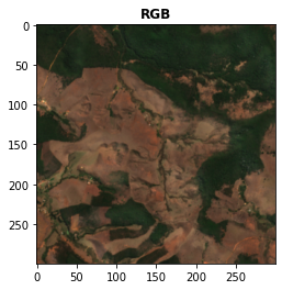
[6]:
<AxesSubplot:title={'center':'RGB'}>
Great! Everything is going great!
Now, let’s convert our normal xarray.DataArray to a rechunked one:
[8]:
da = da.chunk({"band":1,"x":100,"y":100})
Let’s see what we have:
[9]:
da
[9]:
<xarray.DataArray (band: 4, x: 300, y: 300)>
dask.array<xarray-<this-array>, shape=(4, 300, 300), dtype=float64, chunksize=(1, 100, 100), chunktype=numpy.ndarray>
Coordinates:
  * band     (band) <U3 'B02' 'B03' 'B04' 'B08'
Dimensions without coordinates: x, y
- band: 4
- x: 300
- y: 300
- dask.array<chunksize=(1, 100, 100), meta=np.ndarray>
Array Chunk Bytes 2.75 MiB 78.12 kiB Shape (4, 300, 300) (1, 100, 100) Count 36 Tasks 36 Chunks Type float64 numpy.ndarray - band(band)<U3'B02' 'B03' 'B04' 'B08'
array(['B02', 'B03', 'B04', 'B08'], dtype='<U3')
Nice! Now let’s compute the NDVI:
[11]:
NDVI = spyndex.computeIndex("NDVI",{"N": da.sel(band = "B08"),"R": da.sel(band = "B04")})
Let’s check our result:
[12]:
NDVI
[12]:
<xarray.DataArray (x: 300, y: 300)>
dask.array<truediv, shape=(300, 300), dtype=float64, chunksize=(100, 100), chunktype=numpy.ndarray>
Dimensions without coordinates: x, y
- x: 300
- y: 300
- dask.array<chunksize=(100, 100), meta=np.ndarray>
Array Chunk Bytes 703.12 kiB 78.12 kiB Shape (300, 300) (100, 100) Count 81 Tasks 9 Chunks Type float64 numpy.ndarray
It’s a chunked xarray.DataArray! This means that it is not computed yet, so let’s compute it!
[13]:
NDVI = NDVI.compute()
Now, if we take a look at our NDVI, you’ll see that it is already computed! And it was done in parallel with dask!
[14]:
NDVI
[14]:
<xarray.DataArray (x: 300, y: 300)>
array([[0.74305276, 0.75795126, 0.74112076, ..., 0.26035088, 0.25521011,
        0.24128503],
       [0.73163726, 0.72762313, 0.73183055, ..., 0.26452976, 0.29370383,
        0.30510949],
       [0.71619925, 0.71220105, 0.72914046, ..., 0.3265157 , 0.39059464,
        0.48171701],
       ...,
       [0.11111111, 0.1231926 , 0.1231926 , ..., 0.25484352, 0.20737913,
        0.19363998],
       [0.1107078 , 0.11018957, 0.12243702, ..., 0.22382778, 0.19786096,
        0.20110003],
       [0.12105927, 0.10950662, 0.11909037, ..., 0.23674074, 0.23066577,
        0.19771183]])
Dimensions without coordinates: x, y- x: 300
- y: 300
- 0.7431 0.758 0.7411 0.7222 0.7263 ... 0.2582 0.2367 0.2307 0.1977
array([[0.74305276, 0.75795126, 0.74112076, ..., 0.26035088, 0.25521011,
        0.24128503],
       [0.73163726, 0.72762313, 0.73183055, ..., 0.26452976, 0.29370383,
        0.30510949],
       [0.71619925, 0.71220105, 0.72914046, ..., 0.3265157 , 0.39059464,
        0.48171701],
       ...,
       [0.11111111, 0.1231926 , 0.1231926 , ..., 0.25484352, 0.20737913,
        0.19363998],
       [0.1107078 , 0.11018957, 0.12243702, ..., 0.22382778, 0.19786096,
        0.20110003],
       [0.12105927, 0.10950662, 0.11909037, ..., 0.23674074, 0.23066577,
        0.19771183]])
Let’s visualize it!
[15]:
plot.show(NDVI,title = "NDVI")
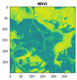
[15]:
<AxesSubplot:title={'center':'NDVI'}>
Amazing!
dask.Series
In Level 3 we worked with pandas.Series. Well, let’s do the same tutorial but now working in parallel again!
Let’s use the pandas.DataFrame that is stored in the spyndex datasets: spectral:
[31]:
df = spyndex.datasets.open("spectral")
As you already know, each column of this dataset is the Surface Reflectance from Landsat 8 for 3 different classes. The samples were taken over Oporto:
[32]:
df.head()
[32]:
| SR_B1 | SR_B2 | SR_B3 | SR_B4 | SR_B5 | SR_B6 | SR_B7 | ST_B10 | class | |
|---|---|---|---|---|---|---|---|---|---|
| 0 | 0.089850 | 0.100795 | 0.132227 | 0.165764 | 0.269054 | 0.306206 | 0.251949 | 297.328396 | Urban |
| 1 | 0.073859 | 0.086990 | 0.124404 | 0.160979 | 0.281264 | 0.267596 | 0.217917 | 297.107934 | Urban |
| 2 | 0.072938 | 0.086028 | 0.120994 | 0.140203 | 0.284220 | 0.258384 | 0.200098 | 297.436064 | Urban |
| 3 | 0.087733 | 0.103916 | 0.135981 | 0.163976 | 0.254479 | 0.259580 | 0.216735 | 297.203638 | Urban |
| 4 | 0.090593 | 0.109306 | 0.150350 | 0.181260 | 0.269535 | 0.273234 | 0.219554 | 297.097680 | Urban |
Here you can see the classes stored in the class column:
[33]:
df["class"].unique()
[33]:
array(['Urban', 'Water', 'Vegetation'], dtype=object)
Each column of the data frame is a pandas.Series data type:
[34]:
type(df["SR_B2"])
[34]:
pandas.core.series.Series
Everything great, right?
Now, let’s create a dask data frame:
[35]:
df = dask.dataframe.from_pandas(df,npartitions = 10)
Let’s see what we have:
[36]:
df
[36]:
| SR_B1 | SR_B2 | SR_B3 | SR_B4 | SR_B5 | SR_B6 | SR_B7 | ST_B10 | class | |
|---|---|---|---|---|---|---|---|---|---|
| npartitions=10 | |||||||||
| 0 | float64 | float64 | float64 | float64 | float64 | float64 | float64 | float64 | object |
| 109 | ... | ... | ... | ... | ... | ... | ... | ... | ... |
| ... | ... | ... | ... | ... | ... | ... | ... | ... | ... |
| 89 | ... | ... | ... | ... | ... | ... | ... | ... | ... |
| 99 | ... | ... | ... | ... | ... | ... | ... | ... | ... |
That’s a dask data frame! Now, let’s compute our indices!
[37]:
indicesToCompute = ["NDVI","NDWI","NDBI"]
Ready?… Go!
[38]:
df[indicesToCompute] = spyndex.computeIndex(
    index = indicesToCompute,
    params = {
        "G": df["SR_B3"],
        "R": df["SR_B4"],
        "N": df["SR_B5"],
        "S1": df["SR_B6"],
    }
)
Let’s see our result!
[39]:
df
[39]:
| SR_B1 | SR_B2 | SR_B3 | SR_B4 | SR_B5 | SR_B6 | SR_B7 | ST_B10 | class | NDVI | NDWI | NDBI | |
|---|---|---|---|---|---|---|---|---|---|---|---|---|
| npartitions=10 | ||||||||||||
| 0 | float64 | float64 | float64 | float64 | float64 | float64 | float64 | float64 | object | float64 | float64 | float64 |
| 109 | ... | ... | ... | ... | ... | ... | ... | ... | ... | ... | ... | ... |
| ... | ... | ... | ... | ... | ... | ... | ... | ... | ... | ... | ... | ... |
| 89 | ... | ... | ... | ... | ... | ... | ... | ... | ... | ... | ... | ... |
| 99 | ... | ... | ... | ... | ... | ... | ... | ... | ... | ... | ... | ... |
Our result is also a dask data frame! Now, just as we did with the chunked xarray.DataArray, we have to actually compute our indices!
[40]:
df = df.compute()
Now, let’s see what we have:
[41]:
df.head()
[41]:
| SR_B1 | SR_B2 | SR_B3 | SR_B4 | SR_B5 | SR_B6 | SR_B7 | ST_B10 | class | NDVI | NDWI | NDBI | |
|---|---|---|---|---|---|---|---|---|---|---|---|---|
| 0 | 0.089850 | 0.100795 | 0.132227 | 0.165764 | 0.269054 | 0.306206 | 0.251949 | 297.328396 | Urban | 0.237548 | -0.340973 | 0.064584 |
| 1 | 0.073859 | 0.086990 | 0.124404 | 0.160979 | 0.281264 | 0.267596 | 0.217917 | 297.107934 | Urban | 0.271989 | -0.386671 | -0.024902 |
| 10 | 0.109801 | 0.124184 | 0.166369 | 0.202229 | 0.317330 | 0.314731 | 0.237525 | 298.668260 | Urban | 0.221537 | -0.312098 | -0.004112 |
| 100 | 0.022805 | 0.026105 | 0.051735 | 0.034822 | 0.255455 | 0.114627 | 0.054650 | 291.818548 | Vegetation | 0.760074 | -0.663173 | -0.380530 |
| 101 | 0.021856 | 0.024345 | 0.050635 | 0.034341 | 0.270058 | 0.118175 | 0.052354 | 291.423766 | Vegetation | 0.774367 | -0.684215 | -0.391215 |
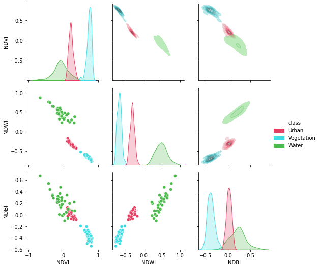
OUR INDICES! COMPUTED IN PARALLEL! :D
Let’s visualize them!
[42]:
import seaborn as sns
import matplotlib.pyplot as plt
Define some colors for each one of the classes:
[43]:
colors = ["#E33F62","#3FDDE3","#4CBA4B"]
Now, let’s create our gorgeous pair grid!
[44]:
plt.figure(figsize = (15,15))
g = sns.PairGrid(df[['NDVI', 'NDWI', 'NDBI','class']],hue = "class",palette = sns.color_palette(colors))
g.map_lower(sns.scatterplot)
g.map_upper(sns.kdeplot,fill = True,alpha = .5)
g.map_diag(sns.kdeplot,fill = True)
g.add_legend()
plt.show()
<Figure size 1080x1080 with 0 Axes>
Splendid!