Xarray
![]()

Welcome to one of the best levels: Level 4 - spyndex + xarray!
Remember to install spyndex!
[ ]:
!pip install -U spyndex
Now, let’s start!
First, import spyndex and xarray:
[2]:
import spyndex
import xarray as xr
xarray.DataArray
If you’re a Remote Sensing scientist, you have probably worked with xarray and Datasets or DataArrays.
Well, well, well… You wnat to use spyndex with xarray, don’t you?
The answer: YES, it is possible!
Let’s use a xarray.DataArray that is stored in the spyndex datasets: sentinel:
[3]:
da = spyndex.datasets.open("sentinel")
This data array is very simple. We have 3 dimensions: band, x and y. Each band is one of the 10 m spectral bands of a Sentinel-2 image.
[4]:
da
[4]:
<xarray.DataArray (band: 4, x: 300, y: 300)>
array([[[ 299,  276,  280, ...,  510,  516,  521],
        [ 287,  285,  284, ...,  503,  476,  469],
        [ 287,  292,  288, ...,  454,  411,  337],
        ...,
        [ 502,  508,  520, ...,  683,  670,  791],
        [ 486,  518,  532, ...,  688,  696,  693],
        [ 486,  506,  515, ...,  659,  671,  664]],

       [[ 469,  446,  466, ...,  695,  711,  728],
        [ 469,  437,  469, ...,  683,  694,  666],
        [ 460,  460,  460, ...,  628,  595,  527],
        ...,
        [ 804,  808,  832, ...,  920,  872, 1023],
        [ 787,  803,  822, ...,  890,  882,  871],
        [ 787,  799,  822, ...,  893,  832,  834]],

       [[ 319,  293,  328, ..., 1054, 1090, 1110],
        [ 327,  318,  345, ..., 1044, 1004,  952],
        [ 339,  355,  323, ...,  922,  784,  652],
        ...,
        [1528, 1516, 1516, ..., 1250, 1246, 1420],
        [1470, 1502, 1498, ..., 1316, 1200, 1162],
        [1394, 1480, 1472, ..., 1288, 1144, 1122]],

       [[2164, 2128, 2206, ..., 1796, 1837, 1816],
        [2110, 2017, 2228, ..., 1795, 1839, 1788],
        [2050, 2112, 2062, ..., 1816, 1789, 1864],
        ...,
        [1910, 1942, 1942, ..., 2105, 1898, 2102],
        [1836, 1874, 1916, ..., 2075, 1792, 1747],
        [1778, 1844, 1870, ..., 2087, 1830, 1675]]])
Coordinates:
  * band     (band) <U3 'B02' 'B03' 'B04' 'B08'
Dimensions without coordinates: x, y- band: 4
- x: 300
- y: 300
- 299 276 280 282 281 255 276 314 ... 1986 1969 1997 2100 2087 1830 1675
array([[[ 299, 276, 280, ..., 510, 516, 521], [ 287, 285, 284, ..., 503, 476, 469], [ 287, 292, 288, ..., 454, 411, 337], ..., [ 502, 508, 520, ..., 683, 670, 791], [ 486, 518, 532, ..., 688, 696, 693], [ 486, 506, 515, ..., 659, 671, 664]], [[ 469, 446, 466, ..., 695, 711, 728], [ 469, 437, 469, ..., 683, 694, 666], [ 460, 460, 460, ..., 628, 595, 527], ..., [ 804, 808, 832, ..., 920, 872, 1023], [ 787, 803, 822, ..., 890, 882, 871], [ 787, 799, 822, ..., 893, 832, 834]], [[ 319, 293, 328, ..., 1054, 1090, 1110], [ 327, 318, 345, ..., 1044, 1004, 952], [ 339, 355, 323, ..., 922, 784, 652], ..., [1528, 1516, 1516, ..., 1250, 1246, 1420], [1470, 1502, 1498, ..., 1316, 1200, 1162], [1394, 1480, 1472, ..., 1288, 1144, 1122]], [[2164, 2128, 2206, ..., 1796, 1837, 1816], [2110, 2017, 2228, ..., 1795, 1839, 1788], [2050, 2112, 2062, ..., 1816, 1789, 1864], ..., [1910, 1942, 1942, ..., 2105, 1898, 2102], [1836, 1874, 1916, ..., 2075, 1792, 1747], [1778, 1844, 1870, ..., 2087, 1830, 1675]]]) - band(band)<U3'B02' 'B03' 'B04' 'B08'
array(['B02', 'B03', 'B04', 'B08'], dtype='<U3')
The data is stored as int16, so let’s convert everything to float. The scale: 10000.
[5]:
da = da / 10000
You can easily visualize the image with rasterio:
[6]:
from rasterio import plot
Let’s visualize the RGB bands:
[7]:
plot.show((da.sel(band = ["B04","B03","B02"]).data / 0.3).clip(0,1),title = "RGB")
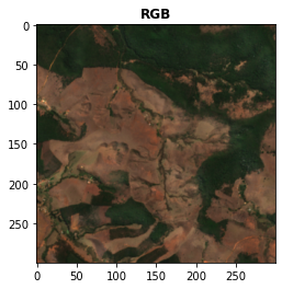
[7]:
<AxesSubplot:title={'center':'RGB'}>
Beautiful image! Now, let’s compute the NDVI for this image (we already know the bands!)
[8]:
NDVI = spyndex.computeIndex("NDVI",{"N": da.sel(band = "B08"),"R": da.sel(band = "B04")})
Let’s check the result:
[9]:
print(f"NDVI type: {type(NDVI)}")
NDVI type: <class 'xarray.core.dataarray.DataArray'>
That’s right: a xarray.DataArray!
Let’s visualize it:
[10]:
plot.show(NDVI,title = "NDVI")
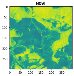
[10]:
<AxesSubplot:title={'center':'NDVI'}>
Now, let’s compute something a little bit harder… the kNDVI!
[11]:
spyndex.indices.kNDVI
[11]:
kNDVI: Kernel Normalized Difference Vegetation Index (attributes = ['bands', 'contributor', 'date_of_addition', 'formula', 'long_name', 'reference', 'short_name', 'type'])
What bands do we need?
[12]:
spyndex.indices.kNDVI.bands
[12]:
('kNN', 'kNR')
What the bear are those!? Those are kernels. How to compute them? Well, spyndex is here to help you!
If you need more information about these kernels, check the Awesome Spectral Indices documentation! ;)
And if you need more info about the kNDVI, check the paper:
[13]:
spyndex.indices.kNDVI.reference
[13]:
'https://doi.org/10.1126/sciadv.abc7447'
You can easily compute kernels with spyndex.computeKernel(). Let’s compute the kNDVI with the RBF kernel:
Note that for the RBF kernel, k(n,n) = 1.
[14]:
parameters = {
    "kNN": 1.0,
    "kNR": spyndex.computeKernel(
        kernel = "RBF",
        params = {
            "a": da.sel(band = "B08"),
            "b": da.sel(band = "B04"),
            "sigma": da.sel(band = ["B08","B04"]).mean("band")
        }
    )
}
With the parameters ready we can compute the kNDVI!
[15]:
kNDVI = spyndex.computeIndex("kNDVI",parameters)
Now, let’s visualize it!
[16]:
plot.show(kNDVI,title = "kNDVI")
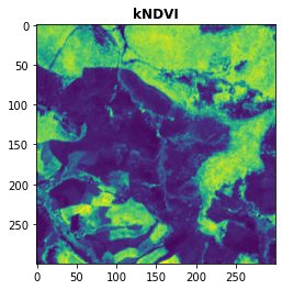
[16]:
<AxesSubplot:title={'center':'kNDVI'}>
And that’s it! You have computed the kNDVI! Amazing, right?