Geopandas

Welcome to the next level: Level 5 - spyndex + geopandas!

Remember to install spyndex!

And also remember to install geopandas! I recommend you to install it using conda!

!pip install -U spyndex

Now, let’s start!

First, import spyndex and geopandas:

import spyndex
import geopandas as gpd

geopandas.GeoDataFrame

In geopandas, each column is a pandas.Series. The exception is the geometry column, which is a geopandas.GeoSeries.

Here we are going to compute spectral indices using pandas.Series data types, but adding them to a geopandas.GeoDataFrame, making them possible to map!

First, let’s create a random sample of reflectances from Sentinel-2. For this, we are going to use Google Earth Engine. Let’s install some useful packages:

!pip install eemont geemap

Then, let’s import them and initialize Earth Engine.

import ee, eemont, geemap

Map = geemap.Map()

Now, let’s use the first image in the Sentinel-2 SR collection and sample 1000 random points from it.

With the eemont package we can mask clouds and scale and offset the image!

poi = ee.ImageCollection("COPERNICUS/S2_SR") \
    .first() \
    .maskClouds() \
    .scaleAndOffset() \
    .sample(numPixels = 1000,geometries = True)

Now, let’s use geemap to convert the samples to a geopandas.GeoDataFrame:

gdf = geemap.ee_to_geopandas(poi)

You can see that the geopandas.GeoDataFrame has the geometry column and the remaining columns are the samples from all bands in the image!

gdf.head()

	geometry	AOT	B1	B11	B12	B2	B3	B4	B5	B6	...	B8A	B9	QA10	QA20	QA60	SCL	TCI_B	TCI_G	TCI_R	WVP
0	POINT (27.29076 26.40036)	0.197	0.1070	0.6306	0.5504	0.1367	0.2429	0.3712	0.4120	0.4322	...	0.4331	0.4570	0	0	0	5	139	248	255	0.695
1	POINT (28.06818 26.58967)	0.198	0.1697	0.5636	0.4815	0.2111	0.3039	0.3790	0.4122	0.4194	...	0.4274	0.4324	0	0	0	5	215	255	255	0.815
2	POINT (27.87679 26.33568)	0.193	0.1670	0.6501	0.5622	0.2118	0.3114	0.4240	0.4666	0.4760	...	0.4990	0.5049	0	0	0	5	216	255	255	0.644
3	POINT (27.04346 26.21331)	0.195	0.1363	0.7335	0.6691	0.1859	0.3268	0.4842	0.5332	0.5514	...	0.5692	0.5823	0	0	0	5	189	255	255	0.624
4	POINT (27.53605 26.84894)	0.194	0.2098	0.6491	0.5494	0.2606	0.3834	0.5202	0.5680	0.5758	...	0.5684	0.5798	0	0	0	5	255	255	255	0.797

5 rows × 22 columns

Now, let’s check the indices to compute: The IRECI and the NDVI:

spyndex.indices.IRECI

IRECI: Inverted Red-Edge Chlorophyll Index (attributes = ['bands', 'contributor', 'date_of_addition', 'formula', 'long_name', 'reference', 'short_name', 'type'])

spyndex.indices.NDVI

NDVI: Normalized Difference Vegetation Index (attributes = ['bands', 'contributor', 'date_of_addition', 'formula', 'long_name', 'reference', 'short_name', 'type'])

spyndex.indices.IRECI.bands

('RE3', 'R', 'RE1', 'RE2')

spyndex.indices.NDVI.bands

('N', 'R')

We need the Red Edge bands from Sentinel-2 plus the Red and NIR bands!

Let’s make a list of the indices:

indicesToCompute = ["IRECI","NDVI"]

Now, let’s compute the indices and add them directly to our geopandas.GeoDataFrame:

gdf[indicesToCompute] = spyndex.computeIndex(
    index = indicesToCompute,
    params = {
        "R": gdf["B4"],
        "RE1": gdf["B5"],
        "RE2": gdf["B6"],
        "RE3": gdf["B7"],
        "N": gdf["B8"]
    }
)

You can see that the indices were added as new columns!

gdf.head()

	geometry	AOT	B1	B11	B12	B2	B3	B4	B5	B6	...	QA10	QA20	QA60	SCL	TCI_B	TCI_G	TCI_R	WVP	IRECI	NDVI
0	POINT (27.29076 26.40036)	0.197	0.1070	0.6306	0.5504	0.1367	0.2429	0.3712	0.4120	0.4322	...	0	0	0	5	139	248	255	0.695	0.073747	0.097496
1	POINT (28.06818 26.58967)	0.198	0.1697	0.5636	0.4815	0.2111	0.3039	0.3790	0.4122	0.4194	...	0	0	0	5	215	255	255	0.815	0.045786	0.070281
2	POINT (27.87679 26.33568)	0.193	0.1670	0.6501	0.5622	0.2118	0.3114	0.4240	0.4666	0.4760	...	0	0	0	5	216	255	255	0.644	0.066105	0.091688
3	POINT (27.04346 26.21331)	0.195	0.1363	0.7335	0.6691	0.1859	0.3268	0.4842	0.5332	0.5514	...	0	0	0	5	189	255	255	0.624	0.085109	0.097904
4	POINT (27.53605 26.84894)	0.194	0.2098	0.6491	0.5494	0.2606	0.3834	0.5202	0.5680	0.5758	...	0	0	0	5	255	255	255	0.797	0.061128	0.060926

5 rows × 24 columns

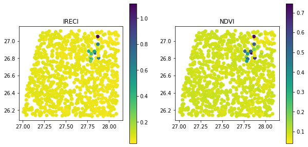
Finally, let’s map the indices!

import matplotlib.pyplot as plt

You’ll see a lot of low values for both indices, that’s because that image is in the desert with some pivot crops!

fig, ax = plt.subplots(1, 2,figsize = (10,5))

gdf.plot(column = 'IRECI',legend = True,ax = ax[0],cmap = "viridis_r")
ax[0].set(title = "IRECI")

gdf.plot(column = 'NDVI',legend = True,ax = ax[1],cmap = "viridis_r")
ax[1].set(title = "NDVI")

[Text(0.5, 1.0, 'NDVI')]

That’s all for now! :) See you in a next tutorial!