Planetary Computer

Do you know Planetary Computer?

Here is a new level!

Level 8: spyndex + Planetary Computer!

Remember to install spyndex and planetary-computer!

!pip install -U spyndex planetary-computer stackstac

And remember to configure Planetary Computer if you have an API key! (If not, that’s okay, just omit this step!)

!planetarycomputer configure

Now, let’s start!

We are going to partially recreate this Sentinel-2 Planetary Computer Tutorial. But now we are going to use spyndex to compute some Spectral Indices!

First, import everything we need:

import spyndex
import stackstac

import planetary_computer as pc
import numpy as np
import xarray as xr
import matplotlib.pyplot as plt

from pystac_client import Client

Let’s open the catalog!

catalog = Client.open("https://planetarycomputer.microsoft.com/api/stac/v1")

Define the IDs of the images we are goingto use:

ids = [
    "S2A_MSIL2A_20200616T141741_R010_T20LQR_20200822T232052",
    "S2B_MSIL2A_20190617T142049_R010_T20LQR_20201006T032921",
    "S2B_MSIL2A_20180712T142039_R010_T20LQR_20201011T150557",
    "S2B_MSIL2A_20170727T142039_R010_T20LQR_20210210T153028",
    "S2A_MSIL2A_20160627T142042_R010_T20LQR_20210211T234456",
]

Search for those IDs in the Sentinel-2 L2A Collection:

search = catalog.search(collections = ["sentinel-2-l2a"], ids = ids)

And sign them with the Planetary Computer API!

items = [pc.sign(item).to_dict() for item in search.get_items()]

Now, let’s use stackstac to create a dask.DataArray from the images!

S2 = stackstac.stack(
    items,
    epsg = 32619,
    resolution = 500,
    assets = ["B04", "B05", "B06", "B07", "B08"],
    chunksize = 256,
).where(lambda x: x > 0, other = np.nan)

Let’s round the time to a daily time scale:

S2 = S2.assign_coords(time = lambda x: x.time.dt.round("D"))

Remember also to scale the collection!

S2 = S2 / 10000

And now let’s check what we have here…

S2

<xarray.DataArray 'stackstac-e6141dd496554095669cb9f3981a0a12' (time: 5, band: 5, y: 227, x: 226)>
dask.array<truediv, shape=(5, 5, 227, 226), dtype=float64, chunksize=(1, 1, 227, 226), chunktype=numpy.ndarray>
Coordinates: (12/44)
  * time                                     (time) datetime64[ns] 2016-06-28...
    id                                       (time) <U54 'S2A_MSIL2A_20160627...
  * band                                     (band) <U3 'B04' 'B05' ... 'B08'
  * x                                        (x) float64 1.362e+06 ... 1.474e+06
  * y                                        (y) float64 -9.075e+05 ... -1.02...
    s2:snow_ice_percentage                   float64 0.0
    ...                                       ...
    gsd                                      (band) int64 10 20 20 20 10
    proj:bbox                                object {699960.0, 809760.0, 8990...
    common_name                              (band) <U7 'red' ... 'nir'
    center_wavelength                        (band) float64 0.665 ... 0.842
    full_width_half_max                      (band) float64 0.038 ... 0.145
    epsg                                     int64 32619

That’s INCREDIBLE! We have our images as a dask.DataArray!

And… if you remember the Dask tutorial, computing Spectral Indices with spyndex and dask is super simple!

Let’s compute the NDVI and the IRECI:

idx = spyndex.computeIndex(
    index = ["NDVI","IRECI"],
    params = {
        "N": S2.sel(band = "B08"),
        "R": S2.sel(band = "B04"),
        "RE1": S2.sel(band = "B05"),
        "RE2": S2.sel(band = "B06"),
        "RE3": S2.sel(band = "B07"),
    }
)

Now, let’s check our result:

idx

<xarray.DataArray 'stackstac-e6141dd496554095669cb9f3981a0a12' (index: 2, time: 5, y: 227, x: 226)>
dask.array<concatenate, shape=(2, 5, 227, 226), dtype=float64, chunksize=(1, 1, 227, 226), chunktype=numpy.ndarray>
Coordinates:
  * time     (time) datetime64[ns] 2016-06-28 2017-07-28 ... 2020-06-17
  * x        (x) float64 1.362e+06 1.362e+06 1.362e+06 ... 1.474e+06 1.474e+06
  * y        (y) float64 -9.075e+05 -9.08e+05 -9.085e+05 ... -1.02e+06 -1.02e+06
  * index    (index) <U5 'NDVI' 'IRECI'

A dask.DataArray! You know what that means… We have to compute the indices!

idx = idx.compute()

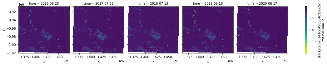
And finally, you can plot the indices! Here the NDVI:

idx.sel(index = "NDVI").plot.imshow(col = "time",cmap = "viridis_r")

<xarray.plot.facetgrid.FacetGrid at 0x7f5fc7c69a90>

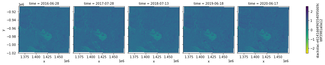
And here the IRECI:

idx.sel(index = "IRECI").plot.imshow(col = "time",cmap = "viridis_r")

<xarray.plot.facetgrid.FacetGrid at 0x7f5fc41ec730>

Wow! :D