Pandas¶

level3

After passing levels 1 and 2, you are ready to start this: Level 3 - spyndex + pandas!

Remember to install spyndex!

[ ]:

!pip install -U spyndex

Now, let’s start!

First, import spyndex and pandas:

[31]:

import spyndex
import pandas as pd

`pandas.Series`¶

We have all worked with pandas. Well, spyndex also works with pandas so you can continue using it! :)

Let’s use a pandas.DataFrame that is stored in the spyndex datasets: spectral:

[59]:

df = spyndex.datasets.open("spectral")

Each column of this dataset is the Surface Reflectance from Landsat 8 for 3 different classes. The samples were taken over Oporto:

[33]:

df.head()

[33]:

	SR_B1	SR_B2	SR_B3	SR_B4	SR_B5	SR_B6	SR_B7	ST_B10	class
0	0.089850	0.100795	0.132227	0.165764	0.269054	0.306206	0.251949	297.328396	Urban
1	0.073859	0.086990	0.124404	0.160979	0.281264	0.267596	0.217917	297.107934	Urban
2	0.072938	0.086028	0.120994	0.140203	0.284220	0.258384	0.200098	297.436064	Urban
3	0.087733	0.103916	0.135981	0.163976	0.254479	0.259580	0.216735	297.203638	Urban
4	0.090593	0.109306	0.150350	0.181260	0.269535	0.273234	0.219554	297.097680	Urban

Here you can see the classes stored in the class column:

[34]:

df["class"].unique()

[34]:

array(['Urban', 'Water', 'Vegetation'], dtype=object)

Each column of the data frame is a pandas.Series data type:

[35]:

type(df["SR_B2"])

[35]:

pandas.core.series.Series

Well, we can use that to compute Spectral Indices with spyndex!

Since we have vegetation, water and urban classes, let’s compute 3 different indices, each one highlighting an specific class: NDVI, NDWI and NDBI:

[36]:

spyndex.indices.NDVI

[36]:

NDVI: Normalized Difference Vegetation Index (attributes = ['bands', 'contributor', 'date_of_addition', 'formula', 'long_name', 'reference', 'short_name', 'type'])

[37]:

spyndex.indices.NDWI

[37]:

NDWI: Normalized Difference Water Index (attributes = ['bands', 'contributor', 'date_of_addition', 'formula', 'long_name', 'reference', 'short_name', 'type'])

[38]:

spyndex.indices.NDBI

[38]:

NDBI: Normalized Difference Built-Up Index (attributes = ['bands', 'contributor', 'date_of_addition', 'formula', 'long_name', 'reference', 'short_name', 'type'])

What bands do we need?

[39]:

spyndex.indices.NDVI.bands

[39]:

('N', 'R')

[40]:

spyndex.indices.NDWI.bands

[40]:

('G', 'N')

[41]:

spyndex.indices.NDBI.bands

[41]:

('S1', 'N')

Green, Red, NIR and SWIR1 bands… easy!

[42]:

parameters = {
    "G": df["SR_B3"],
    "R": df["SR_B4"],
    "N": df["SR_B5"],
    "S1": df["SR_B6"],
}

With our dict of parameters ready we can compute the indices!

[43]:

idx = spyndex.computeIndex(["NDVI","NDWI","NDBI"],parameters)

And, what’s the data type of the result?

[44]:

print(f"idx type: {type(idx)}")

idx type: <class 'pandas.core.frame.DataFrame'>

That’s right! A pandas.DataFrame! Why? Because each computed spectral index is now a column (pandas.Series) of a new dataframe:

[45]:

idx.head()

[45]:

	NDVI	NDWI	NDBI
0	0.237548	-0.340973	0.064584
1	0.271989	-0.386671	-0.024902
2	0.339326	-0.402815	-0.047615
3	0.216278	-0.303482	0.009923
4	0.195821	-0.283852	0.006815

If you want them diectly on the original dataframe as new columns, you just have to play with the code a little bit!

[60]:

indicesToCompute = ["NDVI","NDWI","NDBI"]
df[indicesToCompute] = spyndex.computeIndex(indicesToCompute,parameters)

Now, if you check you original dataframe, you should have the new indices there!

[61]:

df.head()

[61]:

	SR_B1	SR_B2	SR_B3	SR_B4	SR_B5	SR_B6	SR_B7	ST_B10	class	NDVI	NDWI	NDBI
0	0.089850	0.100795	0.132227	0.165764	0.269054	0.306206	0.251949	297.328396	Urban	0.237548	-0.340973	0.064584
1	0.073859	0.086990	0.124404	0.160979	0.281264	0.267596	0.217917	297.107934	Urban	0.271989	-0.386671	-0.024902
2	0.072938	0.086028	0.120994	0.140203	0.284220	0.258384	0.200098	297.436064	Urban	0.339326	-0.402815	-0.047615
3	0.087733	0.103916	0.135981	0.163976	0.254479	0.259580	0.216735	297.203638	Urban	0.216278	-0.303482	0.009923
4	0.090593	0.109306	0.150350	0.181260	0.269535	0.273234	0.219554	297.097680	Urban	0.195821	-0.283852	0.006815

Beautiful! Right?

Now, just for the sake of life, let’s make some visualizations!

[50]:

import seaborn as sns
import matplotlib.pyplot as plt

Define some colors for each one of the classes:

[49]:

colors = ["#E33F62","#3FDDE3","#4CBA4B"]

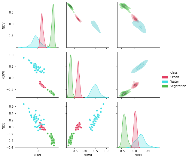
Now, let’s create a gorgeous pair grid!

[64]:

plt.figure(figsize = (15,15))
g = sns.PairGrid(df[['NDVI', 'NDWI', 'NDBI','class']],hue = "class",palette = sns.color_palette(colors))
g.map_lower(sns.scatterplot)
g.map_upper(sns.kdeplot,fill = True,alpha = .5)
g.map_diag(sns.kdeplot,fill = True)
g.add_legend()
plt.show()

<Figure size 1080x1080 with 0 Axes>

Pandas¶

pandas.Series¶

`pandas.Series`¶